We dreamed of decentralised social networks as “email 2.0.” They truly are “television 2.0.”
They are entertainment platforms that delegate media creation to the users themselves the same way Uber replaced taxis by having people drive others in their own car.
But what was created as “ride-sharing” was in fact a way to 1) destroy competition and 2) make a shittier service while people producing the work were paid less and lost labour rights. It was never about the social!
A Review of Apple TV series Constellation (2024)
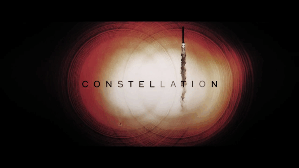
TLDR: Constellation is one of the best science fiction series I have seen in a while. A must watch!
I recently watched the Apple TV series Constellation. The series is gripping, engages you both visually and conceptually and explores some of the deep fears and facts of the human condition.
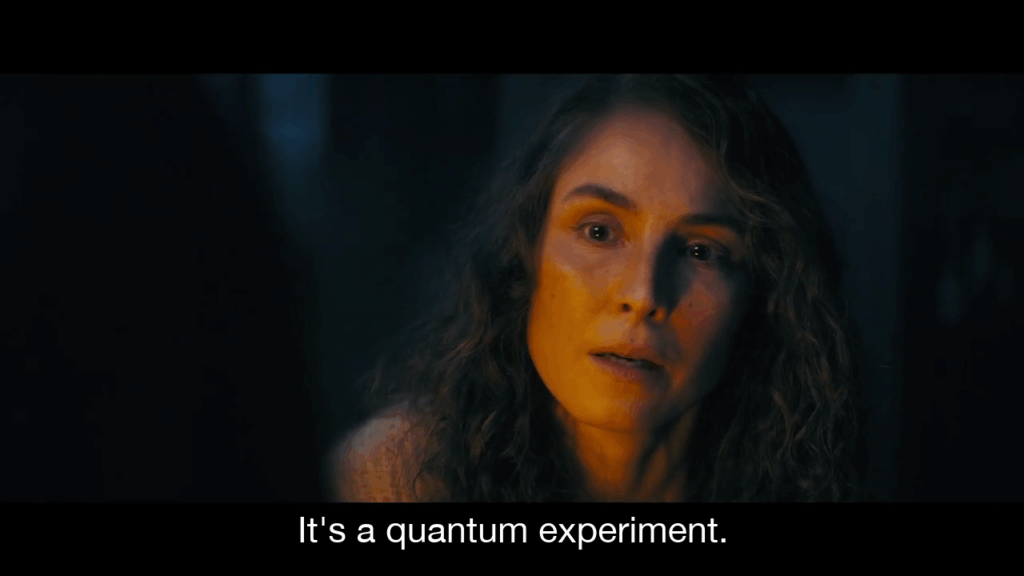
So what is the series about? Well, Jo answers it for us!
Quantum mechanics, developed at the starting of last century, is one of the most counter-intuitive scientific theory that we humans have created. Our notions of “common sense” and our perception of “reality” around us are challenged and refuted in the realm of the quantum. That being said, during its development several gedankenexperiments were done by the pioneers of quantum mechanics. One of the most iconic gedankenexperiment is that was posited in 1935 by German physicist Erwin Schrödinger, the so called Schrödinger’s Cat

The experiment is described as such by Schrödinger
One can contrive even completely burlesque [farcical] cases. A cat is put in a steel chamber along with the following infernal device (which must be secured against direct interference by the cat): in a Geiger counter, there is a tiny amount of radioactive substance, so tiny that in the course of an hour one of the atoms will perhaps decay, but also, with equal probability, that none of them will; if it does happen, the counter tube will discharge and through a relay release a hammer that will shatter a small flask of hydrocyanic acid. If one has left this entire system to itself for an hour, one would tell oneself that the cat is still alive if no atom has decayed in the meantime. Even a single atomic decay would have poisoned it. The psi-function of the entire system would express this by having in it the living and dead cat (pardon the expression) mixed or spread out in equal parts.
It is typical of these cases that an indeterminacy originally restricted to the atomic domain turns into a sensually observable [macroscopic] indeterminacy, which can then be resolved by direct observation. This prevents us from so naïvely accepting a “blurred model” as representative of reality. Per se, it would not embody anything unclear or contradictory. There is a difference between a shaky or out-of-focus photograph and a snapshot of clouds and fog banks. (link)
Stated thus, it questions the very nature of our understanding of reality as seen with our macro senses. How do we understand this? Can the living AND the dead cat exist at the same time? According to the law of excluded middle in our logical system, we assume that proposition is true OR its negation is true. This principle is fundamental in classical logic and asserts that there are no other truth values beyond true or false. So how could the cat exist in both the states: dead AND alive? How do we understand and interpret phenomenon?
There are several interpretations of the cat paradox depending on one’s worldview. The Copenhagen interpretation, one of the more widely accepted interpretations amongst physicists, posits that a measurement results on only one state. This interpretation does not provide an “explanation” for the state of the cat while the box is closed. When the box is not opened, the wave function description of the system consists of a superposition of the states “decayed nucleus/dead cat” and “undecayed nucleus/living cat”. An observer can only assert a statement about the cat only when the box is opened. Thus we can say that the state of the system remains indeterminate, superposition of possible states. The very act of observation collapses the wave function to one of the possible states. Thus observing a system makes the realisation of states possible.
Another way to look at this is the so called many worlds interpretation (MWI) posited by Hugh Everett in 1957. In this interpretation it is posited that there is a universal wave function and in contrast to the Copenhagen interpretation there is no collapse of the wave function. This implies that all states whose superposition creates the wave function are physically realised, but in different “worlds”. What does this mean? The many-worlds interpretation implies that there are many parallel, non-interacting worlds. MWI views time as a many-branched tree, wherein every possible quantum outcome is realized. MWI’s main conclusion is that the universe is composed of a quantum superposition of an uncountable or undefinable amount or number of increasingly divergent, non-communicating parallel universes or quantum worlds. Sometimes dubbed Everett worlds, each is an internally consistent and actualized alternative history or timeline.
So given the MWI framework how do we interpret Schrödinger’s cat paradox?
In the many-worlds interpretation, both alive and dead states of the cat persist after the box is opened, but are decoherent from each other. In other words, when the box is opened, the observer and the possibly-dead cat split into an observer looking at a box with a dead cat and an observer looking at a box with a live cat. But since the dead and alive states are decoherent, there is no communication or interaction between them.
When opening the box, the observer becomes entangled with the cat, so “observer states” corresponding to the cat’s being alive AND dead are formed; each observer state is entangled, or linked, with the cat so that the observation of the cat’s state and the cat’s state correspond with each other. Quantum decoherence ensures that the different outcomes have no interaction with each other. Decoherence is generally considered to prevent simultaneous observation of multiple states. (emphasis added)
Thus every observation event, creates as many worlds as there are states in the superposition. And within each world the events follow as they should. In one world the cat is dead in the other it is not.
Now what would happen if these two worlds, which are split by a certain observation, somehow interacted? There is no “common sense” way to understand or interpret this. It screws your way of thinking, there is no “coherent” way to think about this, it is all “de-coherent”. More you think about it more it becomes perplexing. Curioser and curioser….
And this is exactly the idea that is explored in Constellation series!
All is going well abroad the International Space Station (ISS), where cosmonauts from US, Russia and Europe are placed. Swedish ESO cosmonaut Johanna “Jo” Ericsson (played by Noomi Rapace ) is talking to her daughter Alice (played by Davina Coleman and Rosie Coleman) from the space station. At the same time Paul Lancaster (played by William Catlett) of the NASA astronauts is conducting an experiment to find out about a new state of matter which they think should exist in zero gravity. This is the Cold Atomic Laboratory (CAL).
This is where the story begins. The operation of the CAL is the event which blurs the timelines between the two worlds and allow communication and juxtaposition of the persons and ideas across the worlds which is not supposed to happen in the MWI.
The performance of this experiment gives the predicted result, but causes things to go haywire. There is a collision of the ISS with an unknown object which causes several life-support systems to go out of order. The cosmonauts have to perform an emergency evacuation.
In all this chaos, the Paul is critically injured and eventually succumbs to his injuries. Now for the emergency evacuation, the remaining operational module can only fit three cosmonauts. So a decision is made Jo will remain on the ISS, repair the Soyuz 1 module and return to Earth later, while three other astronauts return to Earth. Jo being alone on the ISS suffers hallucinations (or real visions?) and is on emergency power. These hallucinations (visions?) set the tone for the rest of the series. This is some top-class space-horror. I am not giving out the spoilers..
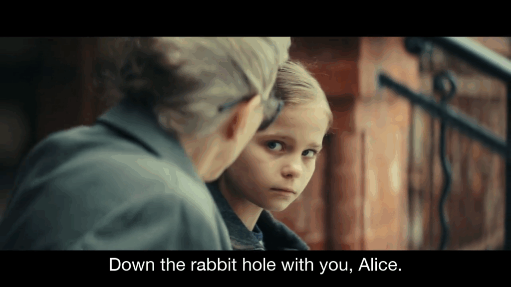
When Jo returns to Earth she feels somethings are different than what she remembered before being up on the ISS. She has been on the ISS for some time (few months). There are strong elements of jamais vu in her experience. For example, Jo remembers her daughter Alice could talk in Swedish, but currently she finds that Alice cannot speak Swedish. Then there are elements of conspiracy theories and Soviet state secrets very seamlessly added to plot. Little things like this take their toll and Jo has a mental breakdown.
Along with Jo, Alice is also finding things disturbing. She also has visions of another Alice in another world, where instead of Paul her mother is dead in the ISS accident. Apart from these two, Bud/Henry Caldera (played by Johnathan Banks) who has designed the CAL experiment also has visions. Thus Jo, Alice, Bud, and Paul are entangled by the event of operating CAL and connections (or cracks?) appear in the divergent worlds between them.
How is this resolved? Do people who are part of these multi-world realities realise that they are in parallel worlds with their counterparts in another world? Well to find out do watch the series!
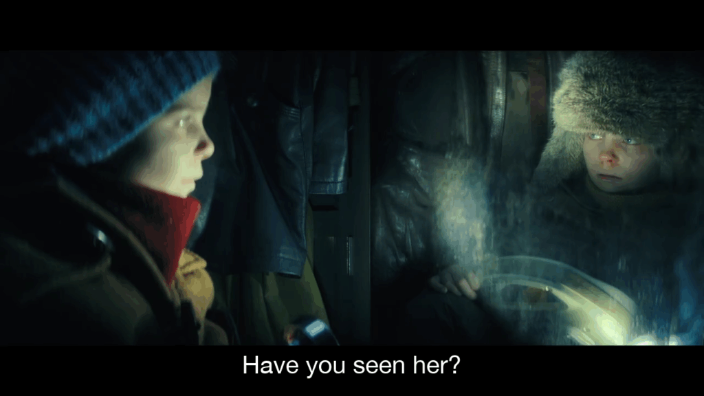
PS: A special appreciation for the role of two Alices played very very ably by the twins Davina Coleman and Rosie Coleman. The sheer sense of helplessness, fear and anxiety portrayed by them when they are trying to find “their mother” is exceptionally brilliant.
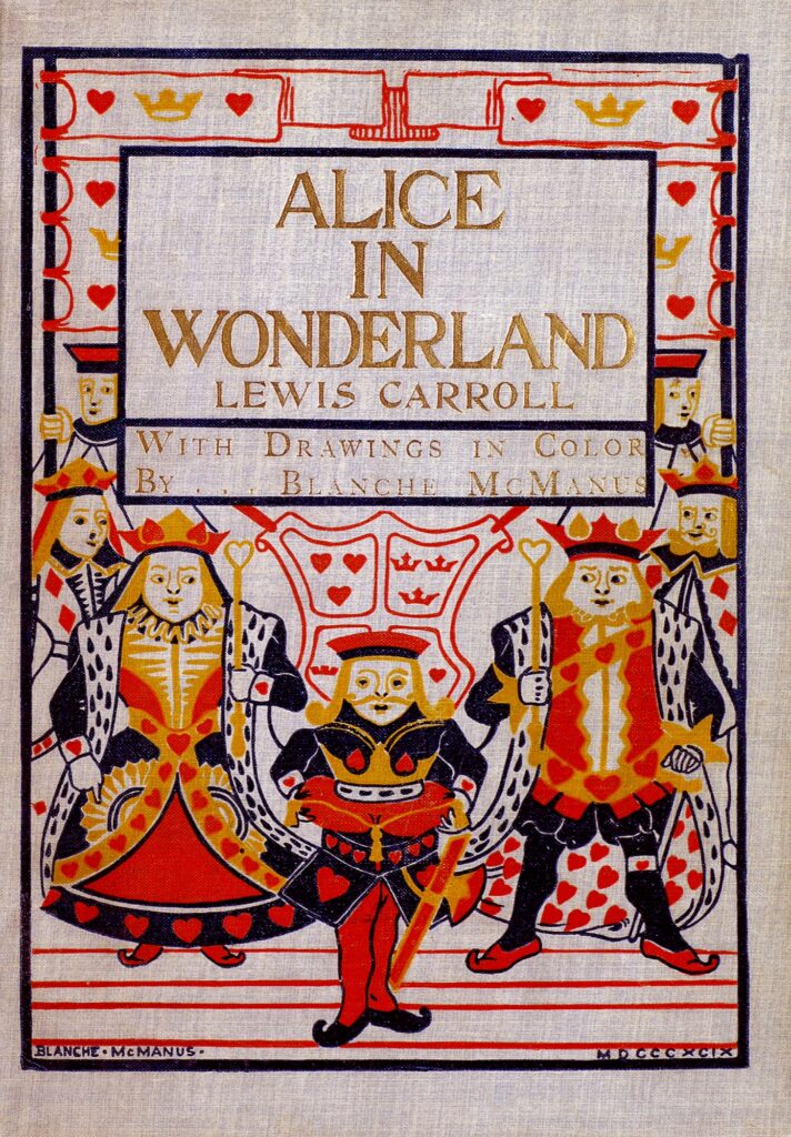
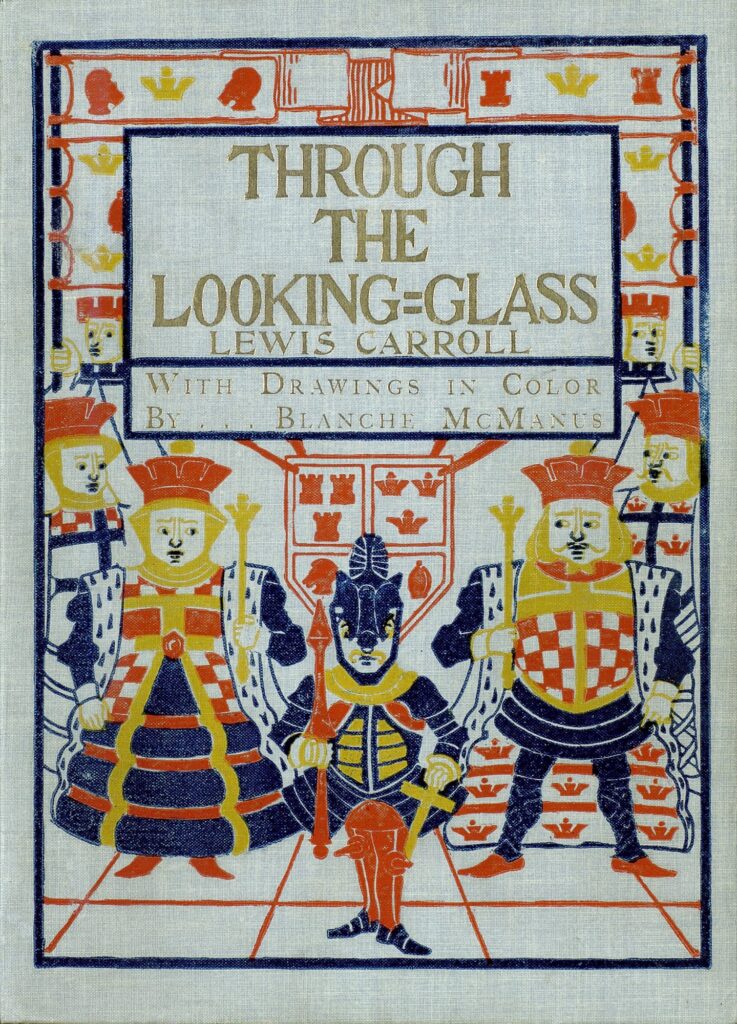
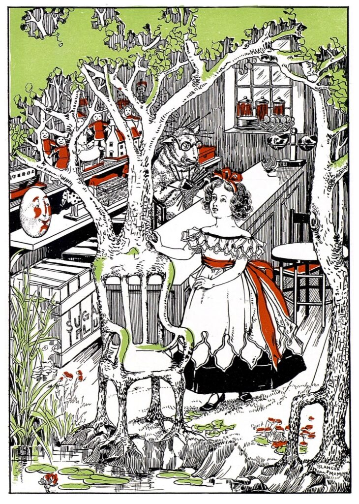
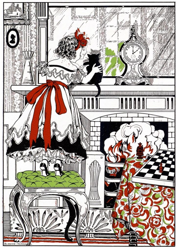
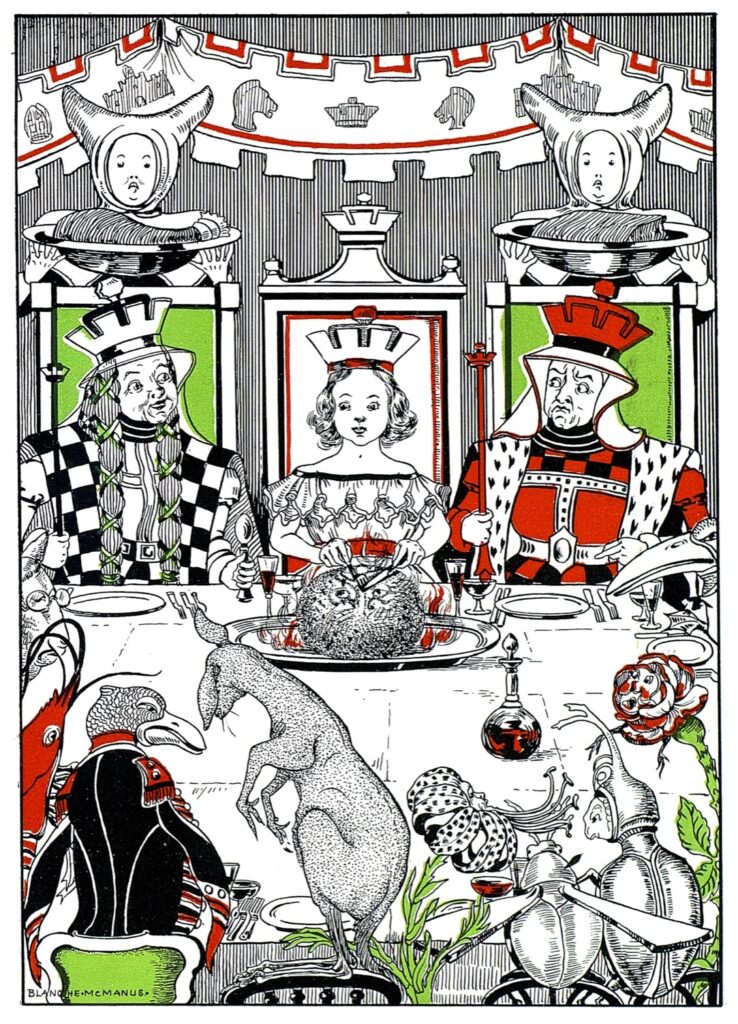
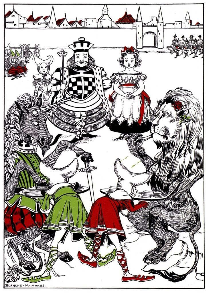
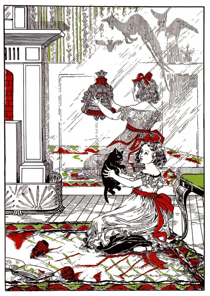
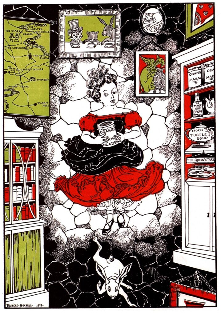
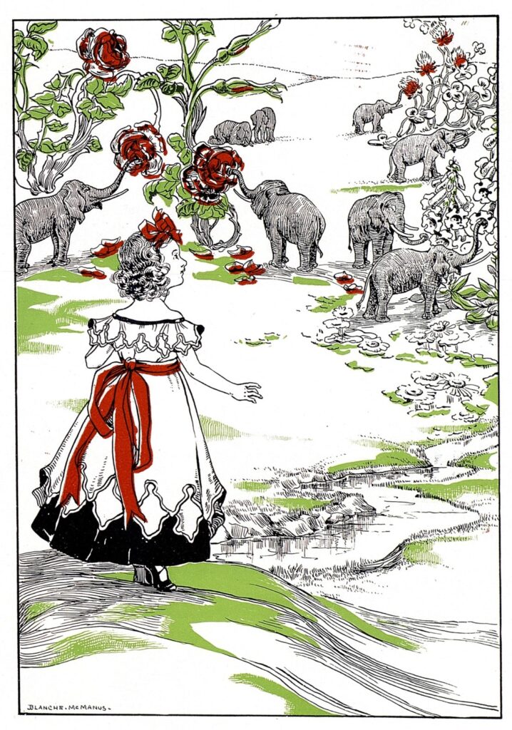
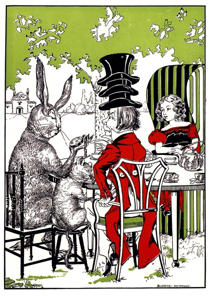
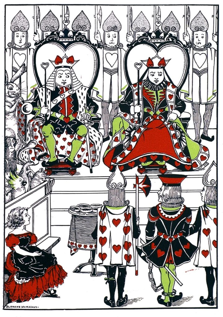
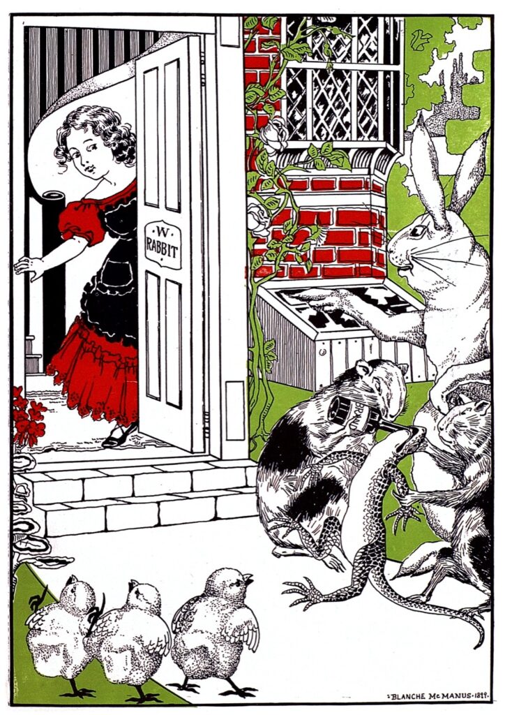
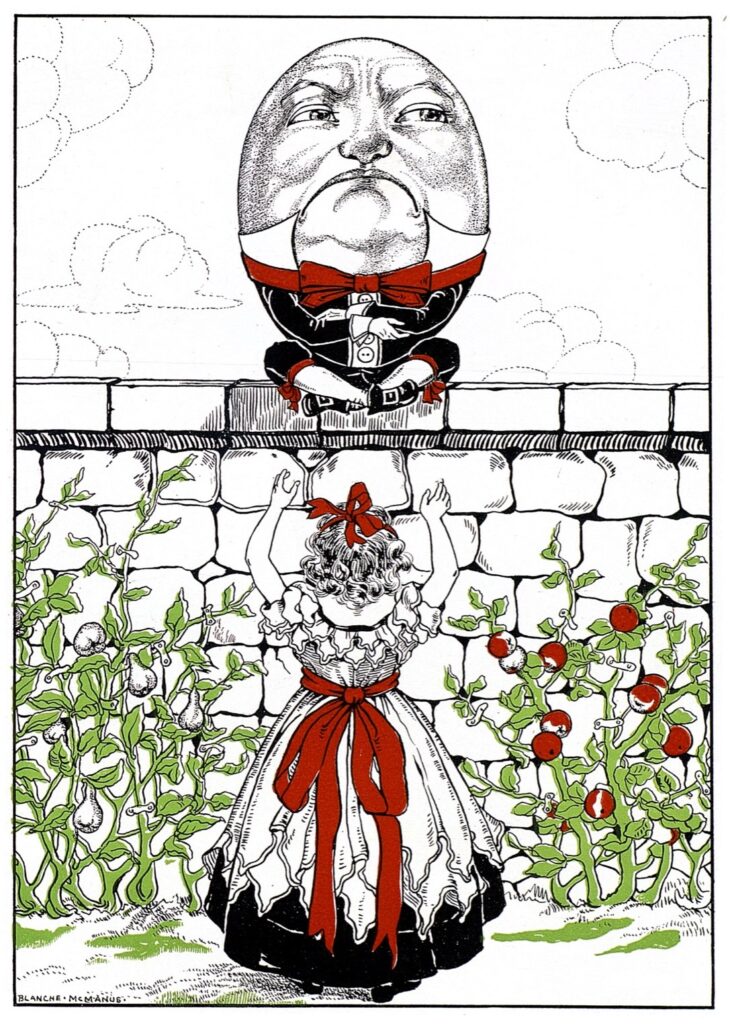
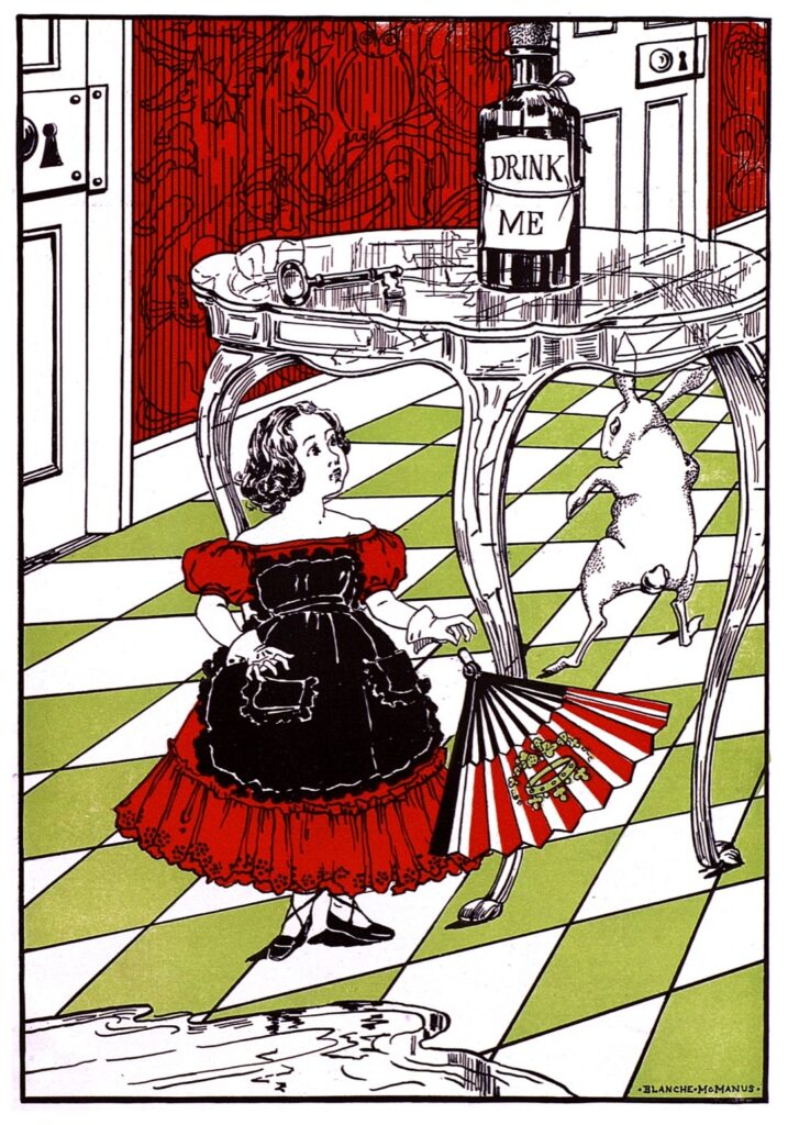
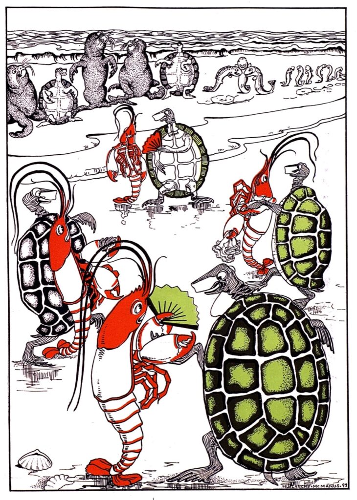
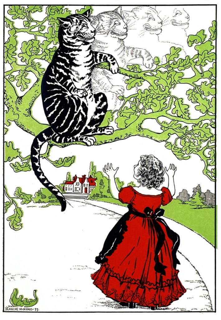
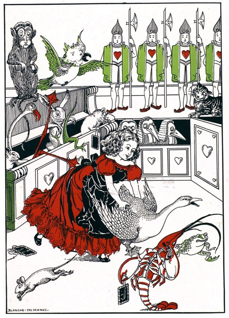
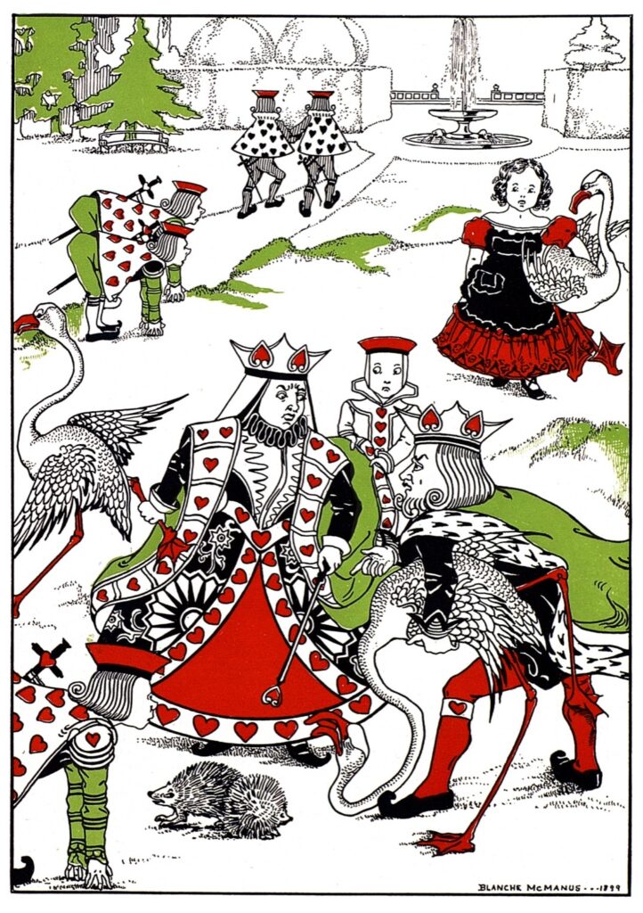
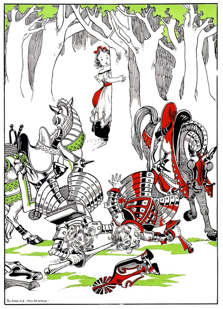
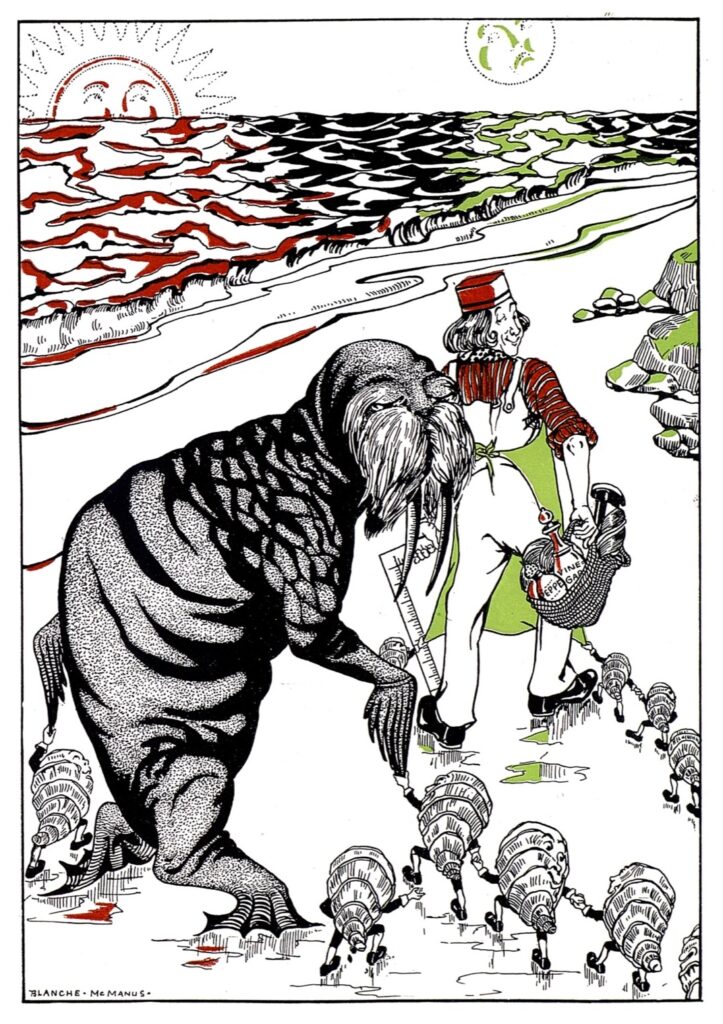
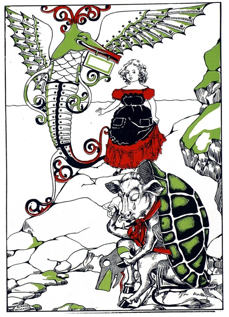
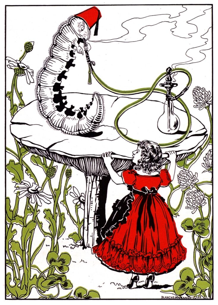
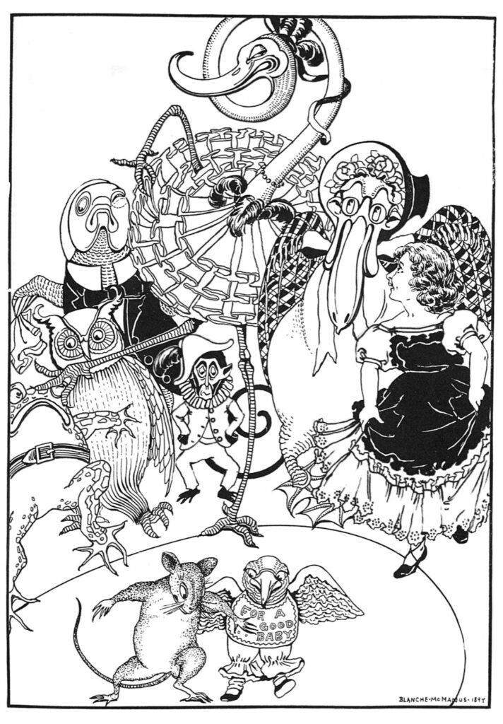
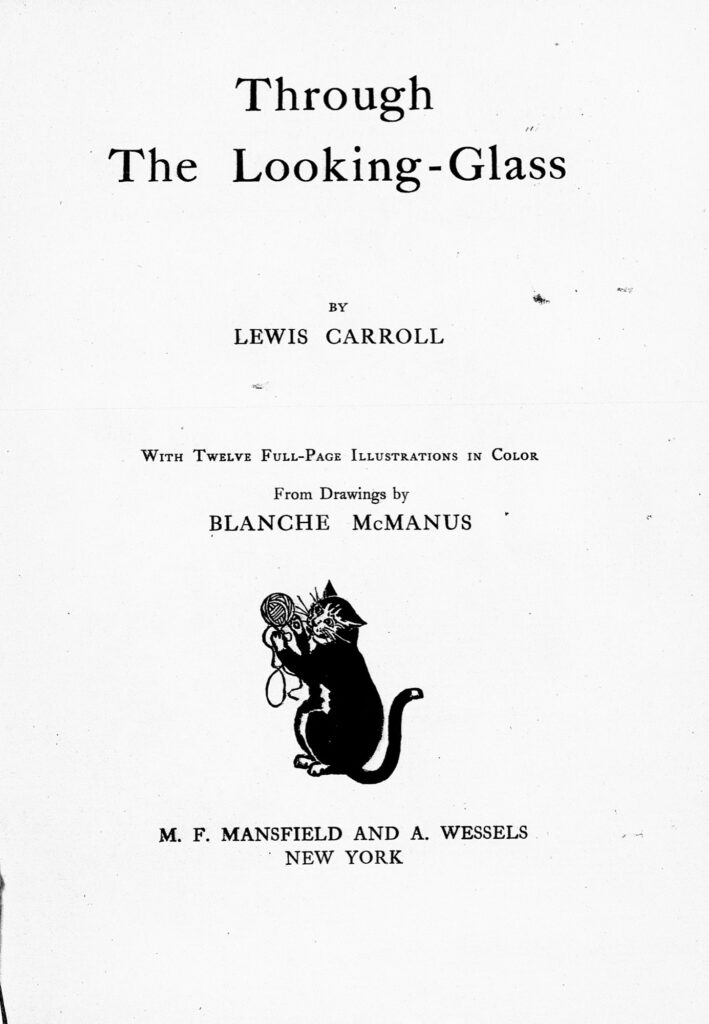
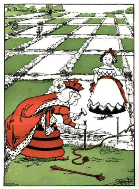
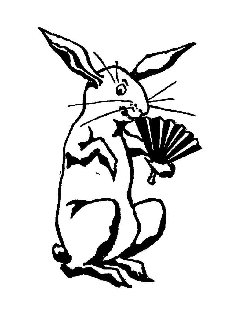
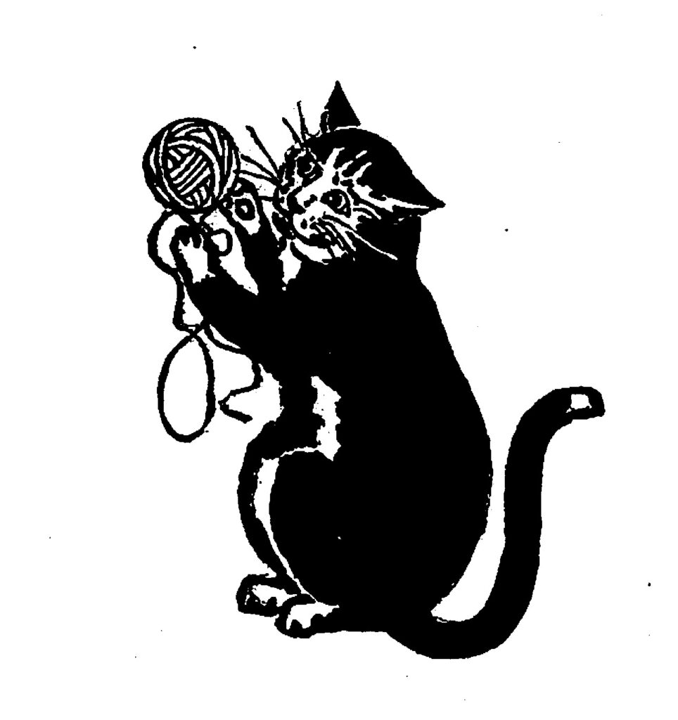
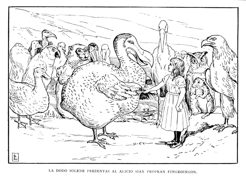
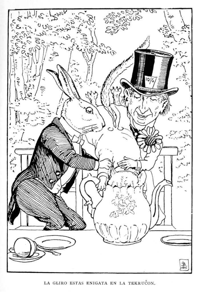
Illustrations for Alice in Wonderland – Part 5 – Blanche McManus
Blanche McManus (1869–1935) was an American writer and artist. She and her husband, wrote a series of illustrated travel books, many of which included information about automobiles which were new at the time. [wiki] She also illustrated both Alice in Wonderland and Through the Looking Glass. In this post we see her illustrations for the two books publishing in 1899. This was the first non-Tenniel illustrated version of the tale [1]. The illustrations are in three colours: red, black and green. There is another set of line drawings by Blanche which I will add later. And another set in which an unknown artist made full colour paintings from the line drawings.
The scans of books are available at University of Florida’s Digital Collections
I have also uploaded the cleaned images to Wikimedia commons in hi-res, search there if you want hi-res images.
(All images in the Public Domain)
![]()
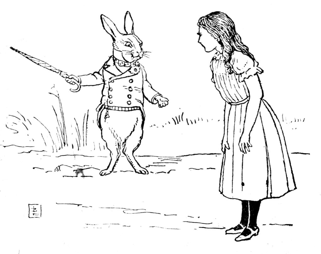
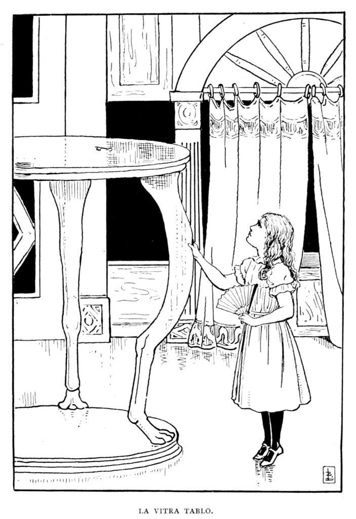
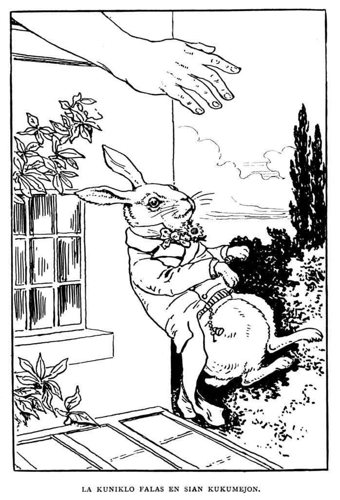
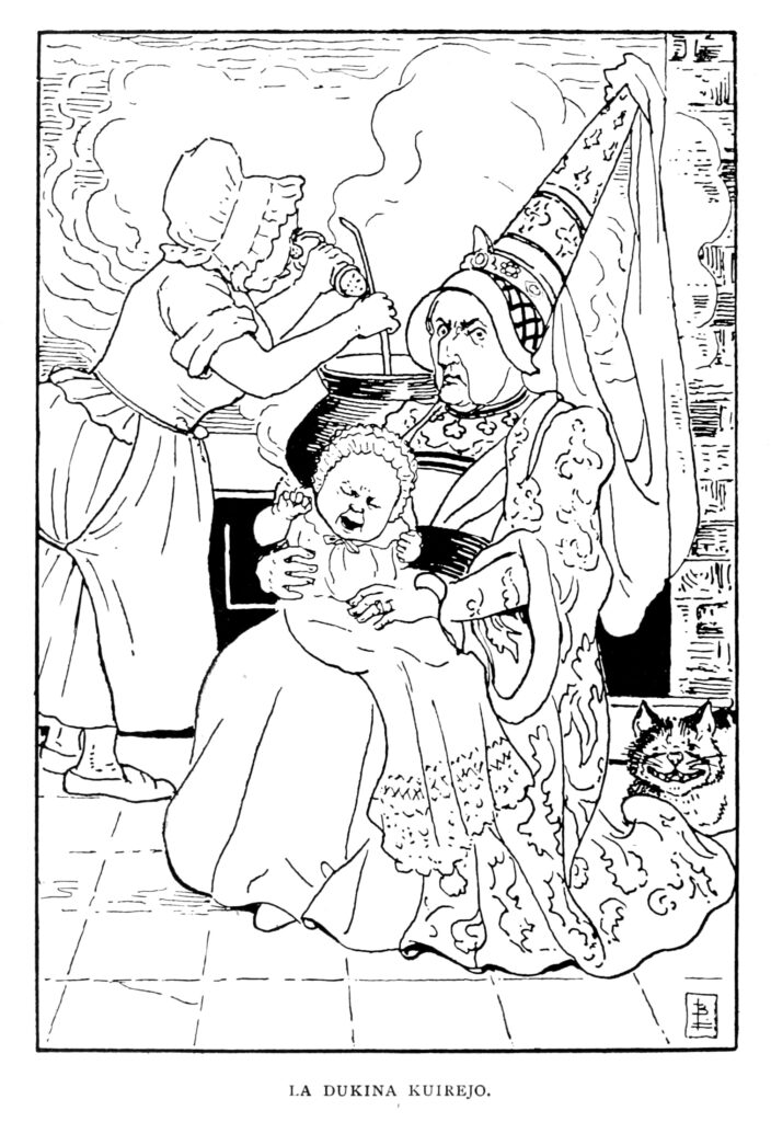
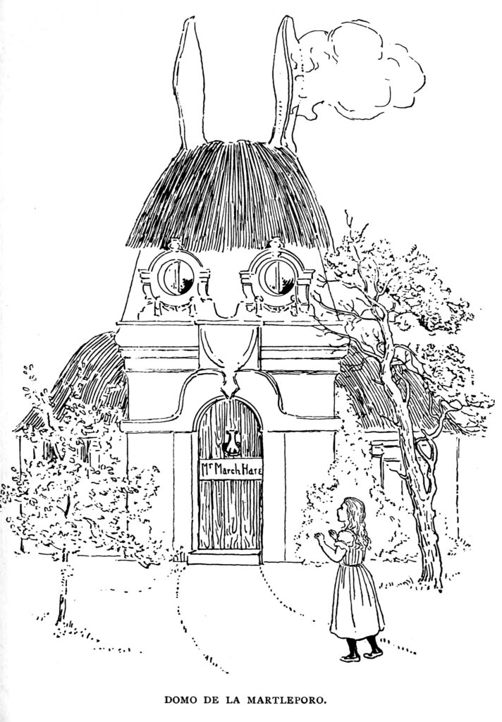
Illustrations for Alice in Wonderland – Part 4 – Brinsley Le Fanu
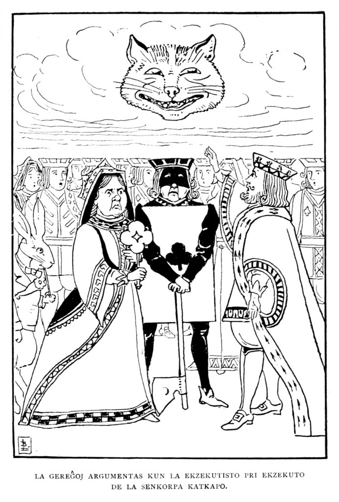
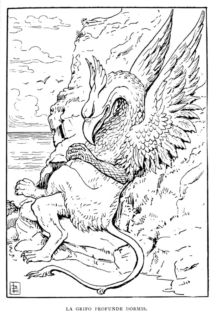
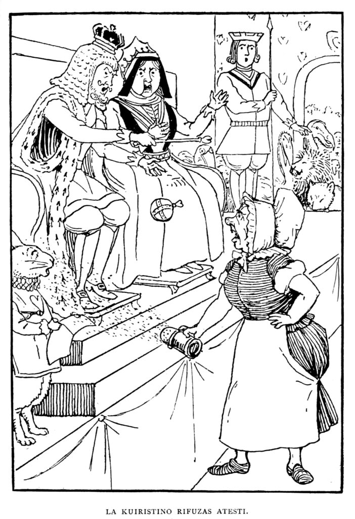
The present post is from a rather peculiar version of Alice’s Adventures translated to Esperanto. The book was published in 1910 by the British Esperanto Association and the translation to Esperanto was done by E. L. Kearney. The illustrations about 10 are by Brinsley Le Fanu (by kind permission of the publisher of Stead’s Prose Classics). So perhaps there is another version with more illustrations by Le Fanu, but I was not able to locate it as such.
All images released under Public Domain CC0.
The Teacher and the Parent

INTRODUCTION
It is very rarely that the teacher in India knows the parents of his pupils. Even when he knows them, it is very rarely that he takes up the problems of his pupils for discussion with them. Still it cannot be denied that mutual understanding and cooperation between the teacher and the parent can go a long way in helping education in schools and developing the personality of the pupil. The teacher has his own view of the child in his care. The child is one of so many students in a class. But to the parent the child is a part of his own self, his future hope. Both these views are partial and one-sided and to some extent blurred. It is only when there is cooperation between the parent and the teacher that the education and development of the child can be understood in their correct perspective.
While in many advanced countries the home and the school are getting closer together and inter-acting for the benefit of children, here in our country no serious attempt has so far been made to get the home and the school influence each other for the advantage of the child. The school and the home in India are separate worlds in themselves. In some cases, however, the teacher is employed by the parents as private tutor for their children. But this does not result in active parent-teacher cooperation. The private tutor is regarded as an appendage, as a part of the staff employed by the home.
The chances of parent-teacher cooperation in the education of children in the hundreds of thousands of elementary and secondary schools in our villages and towns are very slight mainly because of economic factors and the general backwardness of our people. In an overwhelming majority of our schools children receive their education mechanically and regard school-going as part of an established routine, the purpose of which they are unaware. The parent, on the other hand, hardly makes his influence felt in the education of the child. If, however, there is a rare case of a parent trying to take interest in the education of his child and finding out what goes on in the school, the help that he gets from the school is very little.
In the changed circumstances of today, when the character of education has undergone great transformation, parent-teacher cooperation has become essential. Time was when the home itself was the school and the parents and relations of the child were the teachers. In ancient India, on the contrary, the Gurukula was the home of the student. Later on when education became more broad-based, the home and the school became separate entities with very little in common between them. The content of education that was imparted was the be-all and end-all of everything and parents could either take it or leave it. They had no say in the education of the child. All that was aimed at was the gaining of the matriculation certificate by the pupil.
Attempts are now being made to make education more and more child-centred. It has been accepted on all hands that an education which does not encourage the individuality of the child and its development into a well-integrated person is not worth its name. Co-curricular activities, physical education and training in leadership have begun to assume greater importance than mere book-learning. Besides, both parents and teachers have recognised the need to suit instruction to the varied abilities and aptitudes of the children in their charge.
Parents have come to realise in an increasing measure that education is something more than the passing of examinations. Society has become more and more complex. Political emancipation and growing industrialisation have thrown open avenues for leadership and employment. Viewed in this context, the important role that the Indian teacher has to play in society cannot be over-estimated. It is only in very selected schools that he comes across parents who understand the significance and importance of parent-teacher cooperation.
The average Indian parent is yet to realise fully the value of parent-teacher consultations in-the education of the child.
It is in the hands of the teachers to bring the parent round and enlist his active cooperation. In the following pages an attempt is made to explain how the teacher can fulfi his role in this sacred undertaking.
Chapter 1 SCHOOLS AS PARENTS SEE THEM
It is common experience that childhood memories are long-lasting. It would be strange indeed if they did not colour the parent’s approach to those who teach their children. Parents, however successful materially and prominent socially, adopt, in the main, a defensive attitude when they face their children’s teacher. This is not merely true of parents who in their days had been only average students. Even those parents who habitually take pride in their past achievements at school, put on, when they face the teachers of their children, an air of faint aggressiveness, easily detectable as springing from a sense of being on trial. They tend to be over-critical of schools and teachers, which widens the gulf that already exists between the home and the school.
The initiative in bridging this gulf rests with the teacher. He has, so to speak, to break the ice. To do so he has to be understanding; he has to realise that parents see themselves in their children. The teacher has to reassure them and win their confidence. He should be objective, sympathetic and discerning. He should make the school attractive to the child and open the eyes of the parents to the fact that his school has an air of freedom and freshness, which in their own school days they did not experience. If the school is made an interesting place for the child and the teacher adopts the right approach, diffident or defensive or over-critical parents can be brought round to take an active interest in the school in which their children are taught and pay. due heed to the person who teaches them. It is important for the child’s growth that a harmonious relationship is established between its school and its parents, the two component factors that largely determine the character of its world.
It is common experience of teachers that when parents visit schools, one of the oft-heard remarks is that things were very different in their days. Spelling and handwriting and recitation were more conscientiously insisted upon. History and geography were taught with greater precision. In short, what they convey is not very complimentary to the school in which their child is receiving instruction. Normally, the teacher’s reply is not effective; he uses terms like co-curricular activities, progressive education, child-centred teaching, vocational bias, creative expression and so on. All these mean nothing in the absence of a mutual psychological appreciation on the part of the parent and the teacher.
Much of the present dissatisfaction of parents in regard to schools and the reaction of despair in the mind of the teacher can disappear if the teacher, aware of the parent’s picture of the school, tries to change it and paint a new and a truer one in its place. What is happening in our country in the field of education, as in all other fields of national effort, is that both qualitatively and quantitatively, the character of the institutions is changing rapidly.
It is evident that Basic schools, secondary schools, polytechnics and colleges in our country are growing in number with a large intake of students. They are also changing in character and in the objectives they place before themselves. These changes are not, by any means, unwelcome to parents.
On the contrary they are glad, and their reaction is an increased anxiety that their children should benefit in an ever-increasing measure from these changes. It has been the experience of most teachers in the last few years that more parents insist on their children getting technical rather than academic training. Parents wait anxiously to be toid that their children have been chosen for science courses rather than for studies in arts, and the children chosen for the latter very often consider themselves relegated to an inferior intellectual status.
The increasing prominence given to science subjects is a measure of the great change that is taking place in our social outlook. Both parents and teachers understand and recognise the growing importance of Science subjects as natural and inevitable in the circumstances of today. Parents are interested in getting their children admitted to courses in technical studies but they do not concern themselves-and here is the point-with the methods by which instruction is imparted The teacher should take it upon himself to apprise the parent of the content of the courses, the method by which the subjects are taught, the facilities at the disposal of his school, and the potentialities and fitness of the pupils in his charge. He has to convince the parent that the school has the atmosphere and the apparatus to enable him to give the child an all-round instruction, make his life at school a profitable period, and fit him for life after school in the context of the social objectives of the day. He has to make the parent a partner in the adventure which is what educating a growing child is, particularly in these times of change and social progress.
The Indian teacher has it in him to effect a transformation in the attitude of parent to the school. With all the disadvantages he suffers from-and these are not peculiar to this country, and one hopes they will decrease until they cease to be-he has sincerity of purpose and willingness to work.
Therefore, he is more than qualified to address himself to the task of ensuring parent-teacher cooperation.
The amount of such cooperation will vary from institution to institution, school to school, depending upon the peculiar conditions of each institution or school. Whatever the conditions, it is absolutely essential that parents and teachers should find opportunities of meeting each other.
They should meet with a desire to understand each other, to obtain a proper appraisal of each other’s problems and to thrash out ways and means of countering them in a manner that will be salutary for the growth of the child in their care. When the parent sees in the teacher a true guiding spirit intent on drawing out the best in the child notwithstanding the inadequacies that beset his task, his attitude becomes friendly. He sets great store by the contact between such a teacher and the child and the benefits that will accrue by the former’s influence on the mind of the child. It is a worthwhile task, an important pre-requisite to the education of the child, which the Indian teacher is fully competent to perform. The move should come from him.
CHAPTER 2 WHAT PARENTS OUGHT TO KNOW
In such Indian schools where parent-teacher cooperation is practicable, the obsession with the immediate and mechanical academic achievement of the student very often bedevils the relationship between parents and teachers. Here the teacher is less responsible than the parents. Schools which can afford the luxury of some kind of individual attention to each student are usually patronised by parents belonging to the more fortunate classes of society. Parents who send their children to such schools can, if they make an effort, understand that social and economic conditions in the country
are so shaping that leadership in professions, success in industrial management or in the administration of institutions will not hereafter depend so exclusively, as they have done so far, on the narrow mechanical achievements at examinations. In proportion to their capacity for such understanding, the demands of parents on the teachers will change.
The teacher can do very little in creating this understanding. It can be created only by those people who are at the helm, who shape the economic and social policies of the country. It is their task to explain to the public as often and as clearly as possible that the value of education in the future will be judged more and more by the kind of citizens it helps to produce. Education should help to create socially useful men and women, alive to their social responsibilities in a Welfare State. This would mean that in order to be a useful citizen in the context of today a person should be both a specialist in some branch of knowledge and at the same time possess a wide general knowledge and strength of character. If this is impressed upon parents by leaders of thought and action, parents will be able to understand what teachers are up against and what is in the interest of their own children.
Understanding of the social factors will have the way for parent-teacher cooperation. Parents should at least have some idea about what learning stands for. There have been many divergent and conflicting views on learning. According to one school of pedagogy, learning is the development of the capacity in the child to respond in the most advantageous manner to the given stimuli. This school of thought assumes that the capacity in the child to respond can be most effectively developed if the act of response gives a sense of satisfaction. There is another school of thought which holds-mainly among those who are experts on education-that learning depends a great deal on the environment of the learner. They hold that whatever is taught to the child should be related to its environment.
The idea is that a child will perceive quicker and make the knowledge that it obtains its own if what is taught has intimate relationship with the actual living conditions that surround it. If competitive habits are to be learnt, the student must be placed in such a group that he feels he also has a chance to win. There is another concept which lays importance on motivation in the learner. The desire to excel is inherent in every individual. This desire for distinction should be promoted, as frustration of this desire will result in the withering away of learning. At the same time too easy satisfaction of any desire is likely to kill initiative.
All these concepts have elements of fundamental truths in them. In the final analysis the worth of all these concepts lies in their practical application. The teacher in the course of his professional training becomes familiar with these concepts and if he is loyal to his vocation and tries to do his best to provide such situations and offer such encouragement as will result in the drawing out of the will to learn from the students in his charge, he will have done his job. But he has certain limitations. He is not the master of the entire time and environment of his students. The real master of the student’s time and environment is the parent. The parent will be able to influence, the capacity of his child to respond to stimuli, to use his environment and to exercise initiative only if he is familiar with the fundamental truths about learning. This is not to say that the parent also should be a teacher in the strictly technical sense of the term.
In any case, very few parents have the time to usurp, so to speak, the functions of the professional teacher. What is important is the parent should be aware and confident that he can get advice from the teacher in regard to how best he can arrange the home for the maximum advantage of the child. He can help from the home side in establishing a harmonious relationship between the child’s home life and its life at school. Thus begins parent-teacher cooperation. The most that the teacher can do here in so far as parents are concerned is to be ready to otter advice. Beyond that he will naturally be wary. It is a delicate matter for him. Even to offer advice sometimes is not easy. But it is clear that if the education of the child is to be worthwhile at all, parents should be knowledgeable and understanding and teachers devoted to their work and their charge.
Parents’ Notions of Intelligence
Parents form their own notions about the intelligence of their children. Very often we hear parents referring to one of their children as the ‘dud of the family’. ‘Intelligence quotient’ and the letters ‘I.Q.’, though not properly understood have gained common currency in our day. Teachers too use these terms loosely, in place and out of place. “Lacking in intelligence” and “an intelligent student” are stock remarks that teachers write on the progress cards. Let us now attempt to find out what “intelligence” really and truly connotes.
We know only too well that the property termed as intelligence cannot be separated from the child for a correct definition. It is an all-inclusive word, denoting ability, capacity, power and adaptability. A recent definition of intelligence is that it is the ability to undertake activities that are characterised by difficulty, complexity, abstractness, economy, adaptiveness to a goal, social value and the emergence of originals, and to maintain such activities under conditions that demand concentration of energy and a resistance to emotional forces.
The above definition by George D. Stoddard in his book, “The Meaning of Intelligence”, should help both parents and teachers not to use the word so lightly as they do it today.
Both heredity and environment play prominent roles in the acquiring of intelligence. To a large extent, intelligence is an inherited capacity. Through this capacity, it is possible for one to adapt oneself to a suitable environment. In schools, we are more concerned with the role that environment has to play in the possibility of increasing a child’s intelligence. It is environment that provides opportunity and stimulus for
inherited intelligence to develop and function. Both the home and the school do provide such environments. The intelligence of the parents, the intelligence of the teachers, the economic status of the home and of the school, the educational levels of parents and teachers, and situations of the home and the school, all contribute to the environment of the child.
The remark that a particular child has a low I.Q. means almost nothing and it might also mean that the person making the remark is incapable of providing an intelligent environment. The questions whether heredity or environment is the major factor in intelligence remains
as yet unanswered. Parents can justifiably claim that it is environment and teachers will have ample justification too to argue that the child is not intelligent because that is not its family trait. Such a state of affairs can only damage parent-teacher cooperation. So, it is best to believe that intelligence is the product of heredity and environment, each making equal and significant contributions.
As teachers it is our duty to work towards increasing the effective intelligence of the children placed under our care, and this we can do only if we place before them, and surround them with the best possible environmental stimulation. Such conditions, if provided, help also in building up the personality of the children and their emotional stability. Parents should particularly note how the school environment helps to motivate a richer vocabulary, and more correct understanding. If such motivation is not provided, we teachers and our schools are guilty of wasting childhood, and we shall be failing in a sacred social duty.
CHAPTER 3 PARENTS AND CHILDREN
The basis on which parent-teacher relationship should be promoted and the gulf between the home and the school should be bridged is the bond of love which unites parents and children.
Parental love can fill the teacher with confidence in his attempts at cooperation. The teacher knows in advance that the help that he is seeking is only in the interests of the object of the parent’s love. Only in rare cases, parental response will not be forthcoming. The parent cannot but be interested in the teacher who, in turn, is interested in the child. Many of us who see boys and girls in classrooms are not generally conscious of the bond between them and their parents. Each student has his parents at home and incidents that happen at school, trivial or important, get reported at home. If what they hear from their children about their doings at school convinces them that the school has attractions for their chil-dren, they will take some friendly interest in the school. To many of us a student is just a student. The fact that behind the student are his parents who toil for his welfare escapes us.
It is indeed very easy for a teacher to score away a whole line in a student’s notebook with red ink and finally award two marks out of ten for the work done. The teacher might feel irritated at the lack of intelligence shown by the student, but the matter should not end here. He should try and know the sort of home the student comes from, the influences that surround him outside his school. The teacher’s progress reports should not be a routine statement which points out just the bare facts of the student’s performance in a particular paper in an examination. While marks should be given and recorded, the progress report should be based on an observation of the student’s home life, his surroundings, his ability in class and should indicate in what way he has progressed or failed and what he requires if he is to show progress.
It is not selfishness on the part of a parent to want the very best for his child. So teachers who want to break the barrier and bring the home into the school should appreciate the love that binds parents to their children and shape their attitude accordingly. The average parent in India, rich or poor, big or small, is keen to know from the child about happenings in the school. It may be that there are some parents, utterly and selfishly, engrossed in themselves. The large majority are keen to know. how their children are getting on at school, during their most formative years. Though most parents are amateurs in educational methods, they know much more of their own children than we teachers do. We teachers know of their children only as students.
A teacher forms a very good opinion of a class, and it is quite possible that another teacher handling a different subject has a very different opinion of the same class. It may be that teachers have their own opinions about the various students in the same class. But parent’s knowledge of their children as individuals will be far more accurate and dependable than even that of the best teacher. While the teacher can study only one phase of a child’s development, the parent has intimate knowledge of its past life, its likes and dislikes and its innate abilities.
Though the parent alone is in possession of all these details regarding his child, it does not at all mean that he or she alone is the ideal teacher for the child. In many cases we come across parents who do not live up to their responsibilities. Parenthood alone cannot confer on them the rights which they may claim for themselves. There are as many different and difficult types of parents as there are adults in this world. This fast, the teacher has specially to bear in mind in his task of helping the student with the cooperation of his parents.
Students cannot do well in a class if the teacher does not understand them well. Many children are backward in certain subjects due mainly to the fact that the teacher has failed to understand them and their difficulties. The same is the case with parents. The teacher will naturally find it more difficult to understand the parents and their difficulties. The child is young and can be changed, but the adult parent has set convictions.
Once some kind of understanding is established between the teacher and the parent, it becomes simpler for both to discuss the education of the child. Parents should be apprised of the changes that have taken place in educational outlook. Parents should know that ideas on child-care and home management, on elementary and secondary education have undergone a great transformation. Several theories have been welcomed and dismissed like, for instance, Rousseau’s Emile, theories on faculty psychology and the doctrine of formal discipline. All these changes have bewildered the parent and put him at a great disadvantage. Besides, when teachers fail in their task at school, the fashion is to lay the blame on the home without making any attempt to fuse the home and the school. This situation has made even cooperative parents wonder from time to time whether they are doing the right thing for their children. Well-intentioned parents in a state of doubt about their children’s education should be enabled to have experienced advice from responsible teachers.
Parents as Rulers and Inspirers
Of late, as we have seen before, education in India is becoming increasingly child-centred. The first vision of the child is the vision of its parents. Indeed, there are many pro verbs to the effect that parents are the earliest visible manifestations of God. But as the child grows, parents become absolute rulers of the child. There is no doubt that parental control is necessary for a growing child, but the intelligent parent allows free scope for the child’s individuality and growing personality. No rigid rule-of-thumb can be set down as to what extent parents can go in punishing an erring child.
But if there is coordination between the child’s school life and home life, the necessary guidance in the matter of meeting out the correct treatment to the growing child will be available to the parents.
Here we are really up against a problem. There have been many views on the merits and demerits of parental authority. Pestalozzi, for instance, was not very certain where he was to draw the line between freedom and obedience in the education of his own son. This problem of division is not confined to parents alone. It is a problem relating to human life itself and educators both at home and at school have to give it due weight. Much depends on the one hand on the particular child one is dealing with, and on the other on the ability of the teacher and the parent to judge objectively and determine the extent to which they could exercise authority and encourage liberty. There are parents who are natural tyrants and there are also parents who are naturally easy-going.
However, the modern parent will not, it is certain, agree with Rousseau who had this to say of his Emile: “Speak to him of duty, of obedience, he makes nothing of what you say; command him in anything, he will take no notice; but say to him ‘if you will oblige me in this, I will return the favour some other time’, he will immediately hasten to do as you ask, for he likes nothing better than to extend his domination and to acquire rights over you which he knows you will esteem as sacred.” If there be a parent who puts this into practice, he will come in for universal criticism of having utterly spoiled his child. How far then can we accept the suggestion that interference and authority are unwholesome for the child’s developing personality and as such are to be avoided? How far can an average parent go in making everything agreeable to the child? The intelligent parent, in his role as an educator, does, sooner or later, come to understand that if the family atmosphere is one of affectionate trust, all types of control tend to soften themselves into friendly suggestions and children readily respond to them. If care is taken to train the child to proper obedience, to shape its impulses to healthy reactions, duty will become something pleasant to perform. The mixture of parental authority and the child’s liberty should be judicious. This problem that parents face in particular has to be appreciated with discernment and sympathy by the teacher.
The teacher should not scoff at the parent when he puts on an air of authority. The parent knows all about the school from the child which has given the picture as it sees it. The teacher’s feelings about the child and the school should also be made known to the parent. This only the teacher can do. If the parent is in full possession of the facts about the school, both from the point of view of his child and the point of view of the teacher, he will be in a position to cooperate better with the teacher. If there is lack of harmony between what the child is taught at school and the experiences it has in the home, the sufferer will be the child and both the parent and the teacher will have abdicated their duties.
In setting up standards for discipline both the parent and the teacher have a great part to play and they cannot fulfil their role if they part ways and go in opposite directions.
CHAPTER 4 TOWARDS BETTER UNDERSTANDING
Parent-teacher cooperation is based on a, bilateral understanding of a triangular relationship. The parties concerned are the parent, the teacher and the child. The understanding has to centre round the growing personality of the child. It is wrong to assume that the child has no inner conflicts. The youngster at school has deep feelings about many matters. It is dangerous to take a casual view of these feelings. It is the duty of the parent and the teacher to view the feelings of the child discerningly, grasp the emotional upheavals in its mind and help the child in its troubles. If parent-teacher cooperation has to be of value to the child, it is very essential to find out what the child thinks of itself. This may prove to be a difficult task because the child may not be in a position to give cogent expression to its innermost thoughts and feelings.
But an intelligent diagnosis will reveal the psychology of the child. Once the psychological condition of the child is grasp-ed, an intelligent teacher or parent can mould the child on the basis of his understanding. The necessary encouragement or corrective can be given so that the child is able to grow.
A peep into the child’s world will show its thoughts about school, its thoughts about home, its thoughts about teachers and its thoughts about parents, among many other things.
Normally the child thinks very highly of its parents and tries to imitate them in all possible ways. A stage follows when the child begins to criticise parental actions. In between there are also occasions when parents create feelings of irritation, anger and resentment in children. The child is not in a position to know what is good for its growth and what is harmful. Then there is the school about which child has its opinions. It compares conditions at school with the conditions at home. It compares its own home with the home of a class-mate. The ever-widening circle of friends gives rise to social problems and the relative affluence or poverty of its companions, their energies and failings, their ability at school or their backwardness, all these factors influence the child’s mind. The teacher in the course of his instruction should be aware of these factors and in his guidance should take care to give the place of honour to the child’s own home.
Not the least important is the teacher’s attitude to the child’s attitude to him. It should be a matter of great interest to him to know what the child thinks of him and in the event of the child having a bad opinion of him or harbouring some feelings of ill-will towards him, he should try and set the matter right. Nothing is too trivial and if the teacher slurs over these factors thinking that they are of no consequence, it is the child who will suffer. The teacher himself should be on his guard as to how he behaves in the presence of his students.
He may make a casual remark, which the child may take to heart and form, on the basis of that remark, a coloured view of the teacher. It is true that the teacher has to regard the class as a unit and not attach any over importance to any particular individual; but to the extent that each child under his care should receive the fullest benefit of his instruction, it is essential that he should have the growth of each child in mind when he takes the whole class with him. He should have a gift of sympathy and without this sympathy his influence on the growing child will be practically nil and his capacity for cooperation with the parent negligible.
There are different types of parents, although one may say that the average parent in the country is generally a very-accommodating man. But whether a parent is accommodating or otherwise, he still likes some individual attention to be paid to his child. This is natural and the teacher who retorts that he has other children to look after also does not adopt the correct approach. He should expect parents to say that individual attention should be given to their children and point out to them that if his individual attention is to be of any value, parents also should lend a hand and supplement his own efforts. Given that the teacher has the requisite personality and the ability to bring home to the children their responsibility, there will be no difficulty at all in obtaining the cooperation of a majority of parents.
It may be said that in the matter of parent-teacher cooperation extra burden is laid on the teacher as if the teacher does not have his own problems. Economically, professionally and socially, he encounters problems. Besides, even if he is willing not to let these problems worry him unduly and visit parents in their homes with the intention of giving his best attention to the children under his care, things are not too simple for him. It is very likely that the parents in question will take the view that the teacher is angling for some private tuition. On top of all these problems, the periods of teaching work he needs must do, the frightening quantity of correction work to be completed, and the absence of sympathetic understanding on the part of authorities, all these do not make the teacher’s position very enviable.
But conditions are fast changing and the teacher in India is bound to receive better recognition in the years to come. Society is already giving him a nook in its corner. Class-teaching is gradually receding into background as better textbooks and other means of effective teaching and learning are taking the field. The teacher, instead of being the old pedagogue, has begun to assume the role of a director of studies.
For the good of their own children, it is imperative that parents should be aware of this situation. They should view the changes that are now being brought about with hope, and cooperate with the teachers instead of taking up cudgels against them and subjecting the schools to unconstructive
condemnation.
CHAPTER 5 DIVISION OF LABOUR
There is no doubt that in parent-teacher cooperation there is plenty of room for discussion. The discussion should bring out the individual characteristics of the children in a class. Individual differences as in the case of intelligence are the results of heredity and environment. When the teacher takes heredity into consideration, he should be on his guard, for children may be either better or worse than either of the parents, and children of the same parents may vary in their capacities. Instances of an elder brother faring very poorly in a class and the younger one distinguishing himself are very common and teachers have experience of this phenomenon.
Coming to the individual child himself, he may be very good, say, in mathematics, while he may not have the skill to write even a simple composition in English. How far do environments affect individual difference? It is quite possible that children coming from affluent homes are more intelligent than those from poor homes. Very often it is contradicted by the fact that the poor students do much better work through added motivation. If parents are brought together and are made to understand the differences among themselves and the conditions prevailing in their different homes, the resultant comprehension of the situation in so far as individual children are concerned, will lead to beneficial results.
It only conditions were ideal, our classes should not be divided as they are divided now according to differences in age. Individual differences in achievement should be the criterion and classes should be divided into bright, average and backward pupils. In the matter of individual instruction in accordance with. the varied abilities of each pupil, the home has a lot to contribute. The work done at school should be related to the guidance given at home, and the child’s programme both at school and at home should interact and be regulated. Parents. are capable of realising the difficulties that teachers have to face as a result of individual differences in children, if these differences are correctly brought to their attention. Students. who have exceptional ability and show special aptitudes can be encouraged to proceed farther than the limited syllabus of the particular class to which they belong. The slow progress. of the rest of the class need not in any marked degree stultify them. In the same way children who are slow to make progress, in spite of being condemned as dullards, can be, with patience on the part of the teacher and understanding on the part of the parents, rehabilitated till they become confident.
These are the days of planned production and planning for plenty. We have come to realise that there is no work, however stupendous or intricate, that cannot be divided according to a plan. In schools where the aim is to afford opportunities for the pupils to develop a wholesome personality,. the task of education is divided among various teachers who-each in his own way conforming, of course, to a general set pattern-teach various subjects.
The subjects taught, though they may have come to us from the trivium and quadrivium: prescribed by the Greeks of old, do even now have functions. other than their mere content. But the fact remains that as. years advance both teachers and parents tend to belittle the doctrine of formal discipline and greater and ever greater emphasis is being laid on the content. No doubt, we do pay lip-service to the formation of character and discipline. Such an unhealthy trend should not be allowed to continue un-checked. Teachers of languages, arithmetic, science, social studies and art now-a-days undertake to educate children, and such a division of labour, rather than competing with each other, is helping to achieve harmony in the child. When such a division of labour is already in existence, the parent too can be brought into it.
A great educationist once said that the family was like a burning glass which concentrated human sympathies on a point, which was the child. The love of the family stands for human sympathy, and to everyone who comes across it, the budding nature of a child is a matter of deep and tender interest. Parental sympathy and love are the very seeds of morality and among those related by blood, in the narrow circle of family life, due to common aims, common hope and common fears, there springs up a unity and sympathy, based upon affection. In well-regulated families, the individuality of a child finds room for play; but where family life is dis-harmonious, it leaves evil effects on the child. The attitude and outlook of the family, its sense of values-these shape the mental world of the child.
When a family gets a child, the State gets a citizen., The birth of a child, therefore, marks the beginning of parental responsibility as well as the responsibility of the teacher on whom will fall the lot of educating the child. In cases where parental responsibilities have been neglected and as a consequence the child pays the price by developing into an antisocial being, the society does not deny the right of the State to sentence the child to a term in a Borstal school. The conclusion, therefore, is inescapable that mere schooling alone is mot education. The home is the real educator. Schools should open home fronts, in them and parents must be induced, if not compelled, to shoulder their responsibilities as co-educators.
CHAPTER 6 INTERVIEWING PARENTS
To the average teacher, the parent is not generally a very attractive person. The parent’s function, to many a teacher, is to harass the schoolmaster by various means. This is due to the fact that this type of teacher is an isolated person who-does not see even his own headmaster, or meet any of his. colleagues and is unable, in any case, to see himself as a parent. He forgets too that the trustees running the school, the local authority in charge of the school and the inspectorate under which the school functions, are all made up of parents. If parent-teacher cooperation is insisted upon, this type of teacher will necessarily have to alter his views and bring himself into constant touch with the parents of the children who are in his care.
While we stress the importance of the influence of the home in the bringing up of the child, we have got to be careful at the same time about attributing undue importance to it. There are bound to be certain homes where such desirable factors as can help the child’s growth may be totally absent, in which case it becomes the teacher’s duty to devise methods on his own and protect his pupils from harm. There are pupils who are naturally anti-social in their behaviour.
Then there are children who are good at studies and in their general behaviour, but have a congenital knack for flouting authority. The teacher, when he comes across these situations, must be prepared to contend with unfavourable home environments. The task is not easy. Nay, it is beset with great difficulties. There have been instances of young, idealistic but inexperienced teachers-whose motives in reforming then pupils cannot be questioned-having unsatisfactory interviews with the parents and frustrated in their attempts, give up the teaching profession altogether. To cite a recent experience, a boy of 14 was suspected of stealing a fountain pen in the class.
His teacher, anxious not to give too much publicity to the incident, went straight to the parent to apprise him of his strong suspicion of the child’s guilt, thereby ignoring the normal practice of bringing the incident to the attention of the headmaster. The parent’s reaction was one of indignation. He was offensive to the teacher, who felt humiliated and made an announcement in the class that he had decided to fast for three days in order to purify the mind of the boy who had stolen the pen. Five minutes later the guilty boy admitted that he had stolen the pen and proceeded forthwith to produce it from his pocket. When this reached the ears of the parent in question, he asserted that his boy had been bamboozled and coerced to do what he did.
To mention another incident, an eleven-year old student, was observed to be in the habit of skipping his classes in the afternoons. The popular belief was that he was frequently to be seen at a nearby cinema. Twice he was punished in the class, with extra detentions, but to no effect. Whenever asked for an explanation, he pleaded indisposition. The matter was brought to the attention of the boy’s parent. Here again the reaction of the parent was not helpful. In fact, the parent upheld his boy’s interest in films and quoted from his own life as a student. He said that he had become a prosperous business man because in his life, as a student, he had realised that there was no point in being a goody-goody boy and had taken upon himself to acquire a thorough knowledge of the world. So it came as no surprise to him that his son had also followed his steps. The teacher who had gone to report was dumb-founded and returned to the school tongue-tied.
A teacher knows only too well that he cannot understand a child’s action until he comes to know the causes behind it.
In the same way while dealing with parents the teacher ought to try and find out the root causes of their reaction to them.
Considerable patience and tact is required on the part of the teacher. He should not mind facing a rebuff or two.
It should also be understood that parents do not necessarily resent the teacher’s good intentions. But whatever be the failings of their children, they are apt to blame someone else for them. This is not unpardonable and is indeed so common that blaming someone else for any unsatisfactory state of affairs covers other aspects of day-to-day life as well, so much so that it will not be possible for the teacher to resolve emotional tensions in a very short time. But the teacher should be able to suggest several practical remedies and capture the understanding attention of the parents.
There is yet another type of parent who neither resents the interference of the teacher nor lays the blame on others for his child’s failings, but simply promises to do whatever necessary himself. He will even express his gratitude to the teacher for his timely intercession-but there his cooperation will end. In such cases the parent’s reluctance to take the proferred help of the teacher is usually due to two possible states.
One is that the parent has already gained experience in dealing with his child’s problems in the home itself and secondly it may be his defence mechanism asserting itself and impelling him not to feel obliged to another person. In this situation, if the teacher is in possession of a thorough analysis of the child’s behaviour and its complexes and difficulties, he will be able to provide opportunities for the parent also to obtain a true insight into the working of the child’s mind.
To sum up, in parent-teacher cooperation, the teacher should bear in mind the following:-
- Realisation and understanding of the parent’s point of view. This entails an insight into the conditions prevailing in the home and the parent’s behaviour.
- A thorough study of the child’s problems and its abilities and individual differences.
- When such necessity arises, the teacher’s willingness and ability to guide the parent and help him emotionally to overcome his sense of inadequacy that has been the result of a series of failures.
To enable such conditions to prevail, there should be many committees of teachers functioning under the guidance of the headmaster or the principal, so that some of the predominant behaviour problems of students may be discussed and solved. Each school should have a set programme of group discussion among parents and at the same time have facilities for individual counselling. Finally, if teachers make available their special abilities and resources ungrudgingly so that the community can utilise them to enhance the personalities not only of the students but also of the parents, then the basic needs of true education can be met and the reward gained in the noble endeavour will be the growth of wholesome personality in children.
CHAPTER 7 PARENTS’ EXPECTATIONS
The average parent in India pays fees for his children and expects the teacher to do the rest. Very often he grumbles that he is not getting his money’s worth. He has only himself to blame, for the remedy lies in his own hands. It is his duty to his children that he should have some idea of the happenings in the school. He can be, if only he would care to be, the most respected inspecting authority.
Idealism and theories apart, the parent wants that his child should be able to make a comfortable living. When the parent expresses such an aim, which the teacher may consider to be purely utilitarian, there is bound to be a conflict. It is up to the teacher not to be led away by doctrinaire and professional educational philosophy.
If a parent is asked why he does not actively participate in discussions on school curriculum and methods of teaching, his answer is that he finds that teachers are not free agents, and that they are the slaves of time-tables and syllabus imposed upon them by some unknown authority. But today progressive schools, and particularly our Basic schools, do have latitude enough for teachers to show their initiative, and this should be brought to the notice of parents, and to some extent, parents’ wishes and suggestions will have to be put into prac-tice. Modern methods in education do enable us to fit in the parents’ requirements concerning utility.
Many parents now believe that education at the Secondary level, that is, after the children have mastered their “three R’s”, is generally inclined to be chaotic. And they know too that they are finally responsible for the later careers of their sons. The advice of teachers at this stage is most likely to be idealistic. At such a juncture, it is not at all difficult to understand why parents tend to consider a teacher’s expert advice to be anything but merely formal, for the parent is anxious about the utilitarian aspect of education.
In this connection, we cannot but recognise a fact. In the various types of schools in India, and particularly in the field of Elementary and State-aided Secondary education, the curricula and methods of teaching are drawn up by people of high academic experience, who unfortunately are not in touch with the common people. The only remedy for such a state of affairs is for the common people, through their spokesmen, the parents, to make their voice heard and this can be done if every school has a Home Front functioning actively in it. Perhaps it is a fact, and a genuine fact too, that many parents fail to get what they have a right to expect from our present sys. tem of Secondary education. We, teachers, have every justification to claim that such a state of affairs is not entirely our fault. Except perhaps in some progressive schools, our hands are tied by too rigid and regimented a system. The parent has every right to protest that efficiency has suffered due to various experiments in education that have been and are being conducted in recent years. There again, rather than protesting from far away, he should make his voice felt inside the citadel, inside the school. Protestations can be most effective, if there is active and purposive parent-teacher cooperation.
Perhaps parents whom we have to deal with cannot be expected to play their role so effectively in the larger context.
Let us meet them, fully realising their status as co-educators when they approach us on minor details. The majority of them are invariably worried about the poor progress recorded by their children at studies. Such parental visits will go a long way in teachers giving greater personal attention to children needing it, and in imbuing a greater sense of self-confidence in the children.
Parents visit schools with the complaint that children are loaded with such an amount of home work that they feel every vestige of initiative in the young ones is knocked out or irreparably damaged. They claim, and sometimes very logically too, that five or six hours at school should be made to devote to books, and at home scope should be found for them to prosecute interests that the children have adopted as hob-bies. Such parents usually are affluent and the children concerned are invariably intelligent. Teachers should not find it difficult, with the cooperation of the authorities concerned, to find a solution for such complaints.
At the same time, there is the parent who points out that present-day schools do not assign enough home work. He is keen that his children should be at work all the time, and it will be seen that his economy is such that it does not allow him to spend anything appreciable for the entertainment of his children. A resourceful teacher can easily put such a youngster into the habit of wider reading, or he may encourage the student to do some experiments in the physical or chemical laboratory of the school. Such a measure, while satisfying the parent, will go a long way in the true education of the child too.
There are parents-but their number is small-who wisely consider it a necessity to let the teacher know of some special conditions prevailing in the home. The father may be an officer who has to tour extensively and as such, there is not much of adult male guidance at home. The teacher is requested to let the student know that he is aware of it. Or it may be that either the father or the mother is a permanent invalid and the student has to play the part of a nurse at home. The teacher in such a case is requested to excuse the student for not being able to devote enough time for home work. Such cases can easily be understood by a teacher and all possible tensions obviated in the child’s mind.
Sometimes there is the parent who has made a study of educational psychology and considers himself to be an expert in the education of his child. These are usually difficult customers to deal with. They have to be patiently tolerated, and it may also be that the teacher can learn something from him.
Among such, there are those who claim that methods of teaching practised today, even including the principle of sparing the rod, only help to make children into good-for-nothing milk sops. They proudly proclaim the various instances when they themselves had experienced the slashes of a cane from a great disciplinarian and refer to them as the turning point of their lives. When confronted with such parents, if the teacher is not trained in the art of interviewing parents, there is the likelihood of tempers getting frayed. Such parents like to hear their own talk, and the clever teacher ought not to grudge them the pleasure.
Let us round off this chapter with some important tips to young teachers. In parent-teacher consultation and coopera-tion, the following points have to be carefully observed if it is to be of benefit to the child:
- Allow the parent to talk voluntarily.
- Do not be too doctrinaire in your own idealism.
- Don’t let the parent have the idea that you know more of the child than he does.
- When you have a suggestion to make, see that there is more than one way open to the parent for the suggestion to be carried out or the advice adhered to.
The home can become a co-educator only if the school sympathises and realises the difficulties that the home has to contend with.
CHAPTER 8 OPEN DOORS TO PARENTS
In the preceding chapters, we have discussed the difficulties and hurdles that have prevented parents from actively participating in the education of their children in schools. Parent-teacher cooperation can be brought into being in all schools in India whether they be village schools or public schools.
Neither will such a cooperation unduly tell upon the difficult financial situation in the country. There will have to be more teachers in schools, for, if teachers are required to participate meaningfully in getting to know of the difficulties of parents, and thereby be of help and guidance to individual students under their care, the present work-load on teachers will have to be reduced. Teachers should have only four teaching periods per day, and on the computation that he will have correction work for an hour, he should have one hour everyday to be devoted entirely to interviewing parents by appointment and going into the individual cases of his students.
The second essential would be that our teacher-training schools and colleges should have parent-teacher cooperation as a compulsory subject in their courses of studies. The Government and other local authorities should recognise parent-teacher associations and give due weight to the decisions arrived at by such bodies. Such associations should have the right to utilise the school building for their discussions and entertainments connected with furthering parental interest in the education of their children.
The fear that may be expressed by many that such rights conferred on parents may develop into naked and bare-faced interference in the day-to-day running of the school is unfounded. Local factions in the community and the misunderstanding and ill feelings among members of the staff may often culminate in the undoing of a school, but the active cooperation of parents in the welfare of their children can bring about only good to the institution.
The following are some methods of putting parent-teacher cooperation into active practice:-
- Progress reports of students at the end of every month indicating not only the child’s achievements in the studies but also bearing upon his cleanliness, sociality, willingness to work in cooperation with other children and other such traits of character, to be sent to the parents; and at the same time inviting suggestions from parents if they have anything to say on the matter.
- Inviting parents to witness physical training displays by children and tournaments in various games. Proficiency gained by a child at a particular game, or special aptitude shown at a particular co-curricular activity, to be brought to the notice of the parent.
- Sufficient notice given to the parent regarding the weaknesses of particular branches of learning, so that the annual promotion or detention card will not be sprung on the parent as a surprise. When the weakness of a child is being indicated to the parent, steps taken by the school to remedy the weakness should be clearly mentioned and the parent advised to do what is expected of him.
- Parents requested to come over and discuss specific issues regarding their children.
- Parents of children of one particular class at a time, invited to have general discussions with the teachers in charge of various subjects in that class. Discussion may centre round textbooks, curricula, medical examination, progress of children, projects undertaken by the class, examinations and various other matters directly pertaining to the welfare of the children.
- Talks by parents. These can develop either into forum discussions or panel discussions. In these, if teachers too take part, the exchange of views may be beneficial to both.
- Celebration of House Days. As the very name implies, it is an attempt to bring the spirit of the home into the school, where the housemaster plays the role of the senior member of the family. The optimum number of students in a house is twenty-five to thirty. It has been very often noticed that inter-house rivalry in school built up on perfectly healthy lines very soon spreads into the home and parents get to know of the doings of almost every house in the school.
The suggestions enumerated above constitute only a drop in the ocean. As civic consciousness and education spread in India, parent-teacher cooperation is bound to come to the fore. But now, the Indian teacher has not only to initiate the beginnings of such a cooperation, but he or she will have to canvass support and encouragement from the co-educators in the homes. The Indian teacher can and will do it.
The Teacher and the Parent by Rabindra Menon
Ministry of Education, Government of India.
1959.
The Quantum Quarrel
The Quantum Quarrel
Characters:
- Niels Bohr: A physicist of profound thought, firm in his interpretation of the quantum realm.
- Albert Einstein: A physicist of equal renown, resolute in his belief that the cosmos is orderly and deterministic.
- Narrator: Sets the scene.
Setting: A dimly lit chamber adorned with celestial globes, chalkboards scribbled with equations, and shelves of dusty tomes. A fire flickers in the hearth.
ACT I, SCENE I
Narrator:
In times when science sought to find its way,
Two minds of genius met to spar and say
Their truths of nature, veiled in mystery deep,
Where particles like shadows dance and leap.
Attend, dear audience, this fateful night,
When Bohr and Einstein clashed in fiery light.
(Enter Niels Bohr and Albert Einstein, pacing the room.)
Einstein:
Good Niels, thy quantum world is but a dream,
A realm where dice are thrown by hands unseen.
Canst thou truly believe in such a jest,
That nature’s laws bend to chaotic jest?
Bohr:
Ah, Albert, dost thou grasp not what I say?
The atom’s heart obeys no mortal sway.
‘Tis not a dice but probabilities,
That rule the quantum realm and set us free.
Einstein:
Free, thou say’st? Nay, bound in shadows thick!
What freedom lies in chaos so oblique?
The moon, my friend, doth surely shine above,
Though none observe her glow with watchful love.
Bohr:
Yet dost thou not perceive the truth I preach?
Reality is shaped by what we reach.
The moon’s bright face, unseen, is but a guess,
Till instruments confirm its bright success.
Einstein:
And thus, to thee, the cosmos doth depend
On fickle minds of men, and their intent?
Shall nature bow before our gaze so frail,
And truths eternal flicker, shift, and pale?
Bohr:
Not frail, dear Einstein, but wondrously vast!
The world’s deep truths in paradox are cast.
The wave becomes a particle when seen;
Before, ‘tis but potential, soft, serene.
Einstein:
(aside)
A puzzle great, and yet my soul rebels.
How canst thou claim that chaos order quells?
(gesturing to the heavens)
If God should play with dice, then all is lost!
What meaning lies in chance, at such a cost?
Bohr:
God’s dice, perhaps, dost roll with subtle grace,
And randomness conceals a hidden face.
Seek not to tame the quantum’s wily dance,
For beauty lies in mystery’s advance.
Einstein:
(grasping Bohr by the shoulder)
Yet beauty, Niels, must in logic stay,
For chaos leads the mind astray.
Deterministic paths must still exist,
Else reason’s light shall fade into the mist.
Bohr:
(stepping back, arms outstretched)
Oh, Albert, dost thou cling to Newton’s frame,
When nature whispers secrets not the same?
The atom sings a song of prob’listic might,
And not all truths must fit thy steadfast sight.
Einstein:
(softening)
Perhaps, dear friend, in this we both agree:
The cosmos vast exceeds what eyes can see.
Yet still I long for laws that ever hold,
For truths unmarred by chance, both clear and bold.
Bohr:
And I, in turn, admire thy steadfast quest,
For order in the chaos manifest.
Mayhap one day, a deeper truth shall rise,
To merge thy vision with my quantum skies.
Einstein:
Till then, dear Niels, we spar as brothers true,
Seeking the nature of the cosmic hue.
Bohr:
A worthy fight, and noble minds engaged.
Come, let us ponder further, though we’ve aged.
(They exit, arm in arm, deep in thought.)
Narrator:
Thus ends the quarrel of these mighty men,
Yet still their words inspire ink and pen.
For quantum truths remain a riddle vast,
And science seeks to solve them to the last.
Curtain falls.
On reducing the science and maths pass marks
Recently Government of Maharashtra introduced a new idea of reducing the passing marks mathematics and science. It is no secret that mathematics is the most hated and dreaded subject in school learning for many students. Over the decades this idea has been reinforced. Only a few “bright” students in the class seem to “enjoy” mathematics in the classroom. And even getting good marks is no guarantee that the students are enjoying or understanding mathematics. They might be just rote learning entire problems and proofs as is and are able to reproduce them in the examinations. Same is true for sciences also. Students will rote learn and reproduce from memory pages and pages of information about a topic, but if you ask them any conceptual questions they are seen lacking. And this is true for teachers as well. Many teachers, even ones with decades of experience, lack much conceptual clarity or depth in the topics they are teaching. They are able to explain(?) how to solve particular problems or flow of process, but an overarching perspective about the subject matter is often found missing.

Me being a science and mathematics educator finds this state of affairs very saddening. There are some hard facts that the science and mathematics education community in India needs to look at. So far they have been conveniently ignoring the proverbial gorilla in the room, or putting a carpet over it. In this post I want to give my perspective on how the science and mathematics education community has largely failed in addressing some fundamental concerns and are rather interested in problems which do not matter for most of the stakeholders and most importantly for the learners who in the end face the burden of their mistakes.
Now of course doing research is a specialisation. I do not want to sound dismissive of the entire enterprise by saying the act of doing research itself is trivial. That is not the case. Though I have my reservations about how educational research is conducted, that will be topic of another post which I have titled Two Dogmas of Educational Research. The research is done with all the necessary precautions and agendas. Proper citations are made, statistical procedures are applied and it is published in prestigious journals in the field. Year after year conferences are held, attended, latest research presented in them and applauded. The conferences are a celebration of of slides no one reads, jargon no one understands, post-presentation questions that never seem to end and networking. All this, when seen from a non-participating third person perspective somehow feels like both work and a party but achieves neither. I mean of course people do benefit from these, but it is more like I scratch your back you scratch mine.
But way most research articles are written they are jargonified to an extent that they will appear jibberish to anyone who is not trained in understanding the jargon. Articles on teacher education, which want to emphasise importance of teacher education, if given to ordinary school teachers to read (who imho are the stakeholders), will most probably go over their heads. From what little I have understood lot of research in education happens for sake of doing research and not for improving the conditions of stakeholders. The only people who generally benefit from this are researchers who get grants and tenures based on this. How this research actually translates to those stakeholders on whose behalf/improvement they do this is not a matter of concern to them. Another way to say this is that in most cases this research has no value outside of the journals they are intended for.
A lot of Indian educational researchers, when they get a chance to abroad choose to do comparative studies between Indian and other classrooms. This I think is the lowest hanging fruit that one can opt for. I mean if qualitative research teaches you anything it is that context is everything. Of course there are going to be differences in the two classrooms, I will be damned if I don’t find any. But is it worth to do such a research? When countless other times it has been done? Its like comparing apples to oranges literally and then elaborating on how apples are red and oranges are well orange in colour. This fetishisation needs to stop. I will come back to this point later.
Now there is something called as the streetlight effect, or the drunkard’s search principle, is a type of observational bias that occurs when people only search for something where it is easiest to look. This is exactly that has been happening in case of science and mathematics education research at least in India. And yet even after several decades of research they can’t find way to teach fractions correctly to children. Researchers continue to find “new” problems flogging this zombie horse to churn out papers. I am not calling the horse dead, because it, like a true zombie, is resurrected as a “problem” by researchers in each paper and proposing for each research grant. If the horse is dead so will be their research and those grants that they want. So it is in a way self-sustaining problem in educational research. The researchers are in ivory towers and don’t want to get their things dirty with murky things in the actual classroom.
And this is happening because they are choosing the wrong problem to target. Simply because some leaders in the West chose to do so. Most Indian researchers are just following their lead, as they have to submit research in these prestigious journals to be part of the community. We need researchers who will identify problems in Indian context and provide solutions within these contexts. A simple example will suffice. While all effort has been on introducing “constructivism in the classroom” with enormous number of researchers engaged in this one way or other. But how do we actually teach our teachers who are supposed to implement this idea at the grassroots level? Are the student-teacher’s classrooms constructivist in nature? NO. They are just ordinary classrooms who are using behaviourist methods to teach them and then we expect these same teachers to be experts in implementing constructivism in the classroom when they had no experience of it during their own training as teachers or otherwise. This is the same pattern that you will see in all educational research. Researchers and curriculum developers in ivory towers (research institutes and universities) have some lofty normative ideas which they shove down the throats of teachers and ultimately those of the learners without understanding the context in which they will be implemented.
Another day I was talking to a math educator who seemed to be convinced that mathematics needs to be taught for support of “mathematical thinking” to students. And for this it was to be divorced from all other subjects and should be taught for itself. In principle (that is on a curricular document) this seems good, but how does this translate to practice? It might be one of the reasons that mathematics is one the most hated subjects in the school. Learners actually fear mathematics. There is a term specifically coined for this mathophobia. Papert talks about it. But was this of concern to that person, apparently not. They were adamant that mathematics does not need support from other subjects. I was instead arguing for a well founded teaching of mathematics in which mathematics and science go hand in hand. More often that not the mathematics and science follow completely different pathways introducing mathematical concepts to learners (as I found during my PhD work), as if they are teaching completely different people, even for the textbooks of the same classroom. Well, historically mathematics developed for solving problems that our ancestors faced, whether it be about business or science. Why can’t we use the same manner to teach mathematics to our children?
A Parable
Once upon a time, in a far away country, there was a community that had a wonderful machine. The machine had been built by most inventive of their people … generation after generation of men and women toiling to construct its parts… experimenting with individual components until each was perfected… fitting them together until the whole mechanism ran smoothly. They had built its outer casing of burnished metal and on one side, they had attached a complex control panel. The name of the machine, KNOWLEDGE, was engraved on a plaque set in the centre of the control panel.
The community used the machine in their efforts to understand the world and to solve all kinds of problems. But the leaders of the community were not satisfied. It was a competitive world… they wanted more problems solved and they wanted them solved faster.
The main limitation for the use of machine was the rate at which data could be prepared for input. Specialist machine operators called ‘predictors’, carried out this exacting and time consuming task… naturally the number of problems solved each year depended directly on the number and skill of the predictors.
The community leaders focussed on the problem of training predictors. The traditional method, whereby promising girls and boys were taken into long-term apprenticeship, was deemed too slow and too expensive. Surely, they reasoned, we can find more efficient approach. So saying, they called the elders together and asked them to think about the matter.
After a few months, the elders reported that they had devised an approach that showed promise. In summary, they suggested that the machine be disassembled. Then each component could be studied and understood with ease… the operation of machine would become an open book to all who cared to look.
Their plan was greeted with enthusiasm. So, the burnished covers were pulled off, and the major mechanisms of the machine fell out… they had plaques with labels like HISTORY and GEOGRAPHY and PHYSICS and MATHEMATICS. These mechanisms were pulled apart in their turn… of course, care was taken to keep all the pieces in separate piles. Eventually, the technicians had reduced the machine to little heaps of metal plates and rods and nuts and bolts and springs and gear wheels. Each heap was put in a box, carefully labelled with the name of the mechanism whose part it contained, and the boxes were lined up for the community to inspect.
The members of the community were delighted. Their leaders were ecstatic. They ‘oohed’ and ‘aahed’ over the quality of components, the obvious skill that had gone in their construction, the beauty of designs. Here, displayed for all, were the inner workings of KNOWLEDGE.
In his exuberance, one man plunged his hand into a box and scooped up a handful of tiny, jewel-like gear wheels and springs. He held them out to his daughter and glancing, at the label on the box, said:
“Look, my child! Look! Mathematics! ”
From: Turtle Speaks Mathematics by Barry Newell
You can get the book (and another nice little book Turtle Confusion) here.
If the researchers and curriculum developers were ever serious about implementing “constructivism in the classroom” first they would start by reforming teacher education programmes to reflect the pedagogy they want to implement. The second important step would be to reform assessments. Its funny and ironic to see researchers and curriculum developers trying to implement constructivist pedagogies in classrooms with behaviorist assessments and then be dismayed over the results from both students and teachers about their understanding of the subject matter. These strategies are just cosmetic ways to cover fundamental issues that plague the educational system. No reform will be possible with such strategies, but who cares as long as their tenures and grants are justified and their names adorn research reports, textbooks and curricula. They are just repeating the mistakes of the past and expect the results to be different, well it is different in each case and reported in a jargonised framework supported by statistical scaffolding but doesn’t lead to any actual changes on the ground. But that is okay for them as they don’t have any skin in the game, whether learners (both teachers and students) don’t change is not going to do them any harm but keep the zombie alive.
So that the point of all this ranting? The point is that the decision to reduce marks for “passing” is the outcome of such ill-visioned policies and agendas by those who were in position to challenge and change status quo. But instead they choose to go the easier way by keeping the problem alive
On almost becoming knowledge/information black hole
Over the years I have accumulated lot of knowledge/information about things which I find interesting. Some of it is obscure some practical. But If you compare what knowledge/information is coming out of it, it is almost negligible. It is all getting stacked up in the wetware of my mind, and it is getting crowded there. There are not many avenues accessible to me right now where such knowledge/information can be given out. And it is not for the lack of trying. Of course there places where such knowledge/information can be added. But I am avoiding contact via the forums where I could be active but I choose not to. I am becoming more reclusive as the time passes and the feel to get validated by others is diminishing.
Another major challenge has been my own procrastination/lethargy and lack of focus and disciplined planning and overarching purpose for such diffuse unconnected morsels of knowledge/information. But that is exactly what it is. The change in focus is so rapid that it is not making beyond the threshold. In an hour I might be reading about Lucy spy ring during second world war, to origins of consciousness, to recent advances in particle physics to concerns about digital-ebook lending to inferential statistics in R to typesetting a peculiarity in LaTeX …. and the list goes on. At other times it is just mindless scrolling of the endless data stream that has become THE feature of our times. This is sync with the Huxelian vision of future, land of plenty for control. Anyone with an internet connection now has more access to knowledge/information than our predecessors just a generation back.
There is more data in the Matrix than we can download.
But for me personally, it is not leading to production as I would have imagined. It is just getting stuck in the proverbial loop, like The Groundhog day, everyday is the same with little variations here and there. It just is not coming out with any sense of accomplishment. Its not that it has been nothing, there have been outputs, but compared to what it should have been it is below minimal. What knowledge/information is coming out is a trickle as compared to the torrents (both literally and figuratively) that are going in. It is like a knowledge/information blackhole, almost nothing seems to come out as
How to make this even? I think the first step, as many more-able peers had advised me during my thesis writing is to keep absolute time for writing and doing things. Also someone had suggested using the Pomodoro method which has helped me in completing deadlines. Perhaps that is what is needed, a bit of discipline and systematic manner in which to channel both the inputs and outputs..
Learning science progresses funeral by funeral
So said one of the founders quantum mechanics Max Planck. But I think this quote applies to other areas of human endeavour as well. I have been working in the area of learning for major part of my adult life. During my own learning, when computers were just getting mainstream (late 1990s and early 2000s) I experienced first-hand how learning experience can be enhanced by proper use of computers. Another aspect of proliferation of computer which are connected to the internet is that you have access to sum of almost all human knowledge available to you. Even 20 years back this was not the case. I remember when I discovered that there are accessible resources about physics on the web, it was almost a revelation. And the resources grow day-by-day, becoming more and more accessible to everyone. Even with a smartphone you can access all the information on the web. Most modern web designers are adopting a mobile first policy.
I have been musing about these impacts on learning experience ever since. But there is a strong opposition to use technology in the classroom. This mostly comes from people in two categories. One is a old lot who grew and learned in a world without accessible technology and other is a younger lot who have weird (read extremist) ideas about teaching and learning. The younger lot is a lost tribe who live on the Eastern pole. Both these two categories of people opposed to use of technology in the classroom think that they are “progressive” and are fighting against “oppressive” technology.
A note on the term “technology”: Here I am using the term “technology” in a narrow sense of computer technology. A more inclusive sense would include blackboards, printed textbooks and the classroom itself as forms of technology.
I will try to present this perspective of opposition to technology in classroom and dismantle them giving a rebuttal. In some cases, the holders of these ideas are beyond redemption, and quote of the Max Planck which is the title of the post applies to them. They will die off and their technophobia will die with them. A newer generation of pedagogues conversant and comfortable with technology will emerge in the next generation and will be in tune with the need of the time.
Let us start with the older lot. Many of the progressive pedagogues grew in India that was deprived of any computer technology. This was the era of many socialist inspired people’s movement which aspired for egalitarian approach to education, particularly the sections of society which are low in socio-economic order. The approach was to enlighten the masses inspired from the socialist ideas. Now till 90s, the computer technology was expensive and its use even in the developed countries was rather limited. And most of the people in the older lot I am talking about did spend their formative and working years in this era.
Now it is not to say that all of the people did not have any contact with computers at all. Some of these inspired people were highly qualified individuals who did their research work in some of the best institutions in the world. Some of them had some experience of using the computers. But computers were never a second nature to them, as they are not to many people even now. And a lot of them never used computer, because in their era it was an expensive technology and hence they didn’t have access to it. Hence it made computer technology an alien artefact for them in that era.
And when computers finally became accessible, their own years of learning new things had long gone by. Some of them did adopt newer computer technology, able to see the potential to transform both learning and dissemination of knowledge, but most didn’t. Apart from the ideological commitment to a “non-computer” approach to learning, I think their own fears and phobia of being unable to learn and use the new technology also played a role in their opposition. This was the situation in early 2000s, which was still acceptable as computer and internet penetration was not good. These pedagogues threw anything to do with computers as too Western (hence sitting on Eastern pole from where every direction is West).
But by 2010, smart phones were becoming more and more common as were the desktop computers and laptops. By 2015, the access to cheap smart phones with fast internet exploded. Now, here were are in the mid 2020s when proliferation of computer devices in the form of smartphones, tablets and laptops is increasing by the day. The dreams of last mile connectivity are not far off.
The Covid-19 pandemic forced us to shift to online classes. Of course, it did have its issues particularly for students who lacked infrastructure in terms of devices and connectivity. But it did show that even with present conditions something is still possible. Yet, people had their doubts. Now its been
Yet, the resistance from the older pedagogues continues. They cannot get away from ideas about computers that were formed 4 decades back, when computers were still primitive and expensive. And they continue to the same arguments even today. Questions like “Have computers reached everyone?” and since they have not we cannot use them. Or they give overarching statements like “The most downtrodden will be neglected in this”. They are like classical physicists who could not accept ideas of modern physics at the turn of the last century.
To objections like these, I have two rebuttals, one is historical-pedagogical and other is on the nature of computer technology in particular. Let us look at the first objection: “Have computers reached everyone?”, of course, they have not! But what about other technologies like the classroom and blackboard? Yes they are technologies! Have they reached everyone? Of course not! But then you don’t give the same arguments, let school reach every child (or every child reach the school) and only then we will allow/accept school as a viable mechanism for learning. And that is something they will never accept, just because they are comfortable/conversant with technology school-classroom-black-board-textbooks. That is a given for them. But even that “technology” has access issues, and comes loaded with challenges of its own for learning. I mean these are the very challenges that many of these pedagogically oriented movements addressed.
So this argument about last-mile connectivity applies to the existing technologies to teaching and learning as well. Why should it be singled out for “computer” technology? This is only because the older lot is not familiar (rather don’t want to accept) with the potential of the computer technology as it would destroy their anachronistic cherished notions of teaching and learning.
Other major assumption in this notion is that the teacher and textbook are the (sometimes the only) source of knowledge, almost an axiom in the Euclidean sense.
Is this why there was so much focus on developing text-based teaching learning materials. But this is no longer true. We now have almost entire sum of human knowledge accessible literally at fingertips to anyone with a connected device. But now with Open Education and internet this is being challenged in a serious way. Added to this is the absolutely disruptive technology of AI bots like chatGPT. Why should learning be limited to a centralised textbook which usually does not take into account the context of learners written by folks sitting in ivory towers, which is not updated for years?
Now we have the technology and appropriate legal licenses to change this by really empowering learners to bypass the filters of textbooks and teachers. But still we are hung on cherished notion of teacher in the constructivist classroom.
Now, I come to aspects of the nature of technology and young learners. The nature of “computer” technology is such that younger learners adapt to it very quickly. They are still in the phase of learning about the world. A very young child given a smartphone will try out everything and figure out how it works (or doesn’t) and start playing with it as if its any other toy. Parents often ask help from their very young children to solve technological challenges they face.
Same is true for teachers. I have seen enough examples during my field work in very rural areas. Learners when exposed to computer technology even for a very short time several were first-generation learners who were using computer for the first time, could out-pace the teacher in using the computer for the task at hand. Now in the traditional approach (even the progressive ones) the knowledge of teacher is almost never surpassed in a teaching-learning setting. The teacher is always the “more-able-peer” in the Vygotskian sense and is considered as an a priori truth. Now, I am not denying that in many senses this is correct, but if you give access to technology to young learners in many cases the need for teacher is bypassed. This is in the true sense that a child constructs knowledge with the only difference being that it is not mediated by the teacher (or even if it is teacher is exactly a mediator). Constructionist microworlds provide excellent examples of such learning by the learners on their own. By denying access to computer technology, this is what is being missed.
Of course there are examples and examples of bad use of technology in the form of PPT/click books etc which is often rightfully criticised. But that is missing forest of the trees. Another point in this regard is that educational technology abhors vacuum, if any technology is not opted by good pedagogy, it will be co-opted by a bad one. So we need to stake claim, otherwise poor pedagogical approaches which just replicate what is done without a computer to be done on a computer. To give Papert’s analogy it would be like attaching a jet engine to a horse-wagon!
Now we come to the younger lot. They typically have grown with technology in their formative years. And as reasearchers and activists they use computers and internet and are familiar with the technologies. Yet they give the same arguments of “oppression” as the older lot. I mean it doesn’t occur to them they are using the same computers for their own work because it suits them. But when it comes to use in the classroom it is not to be used. Double standards much. If they think the computers are oppressive as much, they should stop using it themselves. But then how will they post social media updates on Facebook and Twitter?
The younger generation of people who oppose technology in the classroom fits very well in the category of people without skin in the game (after Taleb). For things they think computer is useful for themselves, they will make full use of it be it data analysis, report writing or other work. But they are not ready to give same concession to children (especially in resource deprived areas) who need such scaffolding more. Instead they want to deprive the children of a learning companion because it does not work with their ideological world view centred at Eastern pole. And some of these same researchers, when it comes to their own children will provide them with computers and tablets for learning. But when it comes to the children who need it more…
I could go on and on.. But you get the point, the opposition is not based on factual aspects but ideological and there too they are on thin ice. But the opposition is waning funeral by funeral and computers are the new normal…
Book Review: Parasite Rex by Carl Zimmer
This is a scary book. I mean it is a very good introduction to how parasites live their life among their hosts and thrive. The book takes look at various parasites and their natural history in terms of evolution and the impact parasites have in the ecology and individuals. How many behaviours in their hosts are manifestation of parasites trying to maximise their chances of getting too they next guy in their life cycles. For example, the malarial parasite plasmodium generates chemical signals that give us fevers at very specific times of the day which coincides with the time when mosquitos are active. From evading the immune system to completely controlling organisms by taking over their nervous system parasites are highly evolved in their way of life.
Zimmer takes a perspective that parasites have a major role in any functional ecosystem and drives the evolution of their hosts as well. Earlier parasites were treated as
Low end ke forms but studies now show his little we know how they work. Almost all wild animals are full of parasites and Zimmer also makes a case that having parasites is a sign of a good ecosystem. They are not organisms in the fringes but rather a driving force across the ecological niches.
Why I said the book is scary is the sheet amount of parasites that can easily enter your body and how little we can do about it. As you read about various ways in which you can get infected leaves you scared.