Stellar Exploratory Data Analysis or How to create the HR Diagram with R


I recently have started to refresh my skills with R programming language. I am doing the  Harvard Course on Data Science on EdX. I am using R Studio for doing all the exercises. In the second part of the course, Visualisation, which is an area of research interest for me, there is an exercise on stars dataset. But this exercise was available only to those who were crediting the course. Since I was not crediting, but only auditing I left the exercise as it is. But after a week or so I looked at the stars dataset. And thought I should do some explorations on this. For this we have to load the R package dslabs specially designed for this course. This post is detailing the exploratory data analysis with this dataset. (Disclaimer: I have used help from ChatGPT in writing this post for both content and code.)

> library(dslabs)

Once this is loaded, we load the stars dataset

data(stars)

Structure of the dataset

To understand what is the data contained in this data set and how is it structured we can use several ways. The head(stars) command will give use first few lines of the data set.

> head(stars)
star magnitude temp type
1 Sun 4.8 5840 G
2 SiriusA 1.4 9620 A
3 Canopus -3.1 7400 F
4 Arcturus -0.4 4590 K
5 AlphaCentauriA 4.3 5840 G
6 Vega 0.5 9900 A

While the  tail(stars) gives last few lines of the data set

tail(stars)
star magnitude temp type
91 *40EridaniA 6.0 4900 K
92 *40EridaniB 11.1 10000 DA
93 *40EridaniC 12.8 2940 M
94 *70OphiuchiA 5.8 4950 K
95 *70OphiuchiB 7.5 3870 K
96 EVLacertae 11.7 2800 M

To understand structure further we can use the str(stars) command

> str(stars)
'data.frame': 96 obs. of 4 variables:
$ star : Factor w/ 95 levels "*40EridaniA",..: 87 85 48 38 33 92 49 79 77 47 ...
$ magnitude: num 4.8 1.4 -3.1 -0.4 4.3 0.5 -0.6 -7.2 2.6 -5.7 ...
$ temp : int 5840 9620 7400 4590 5840 9900 5150 12140 6580 3200 ...
$ type : chr "G" "A" "F" "K" ...

In RStudio we can also see the data with View(Stars) function in a much nicer (tabular) way. It opens up the data in another frame as shown below.

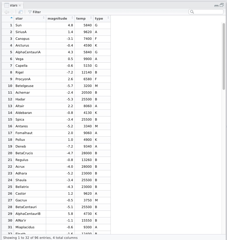
Thus we see that it has 96 observations with four variables, namely star, magnitude, temp and type. The str(stars) command also tells use the datatype of the columns, they are all different: factor, num, int, chr. Let us understand what each of the column represents.

Name of stars

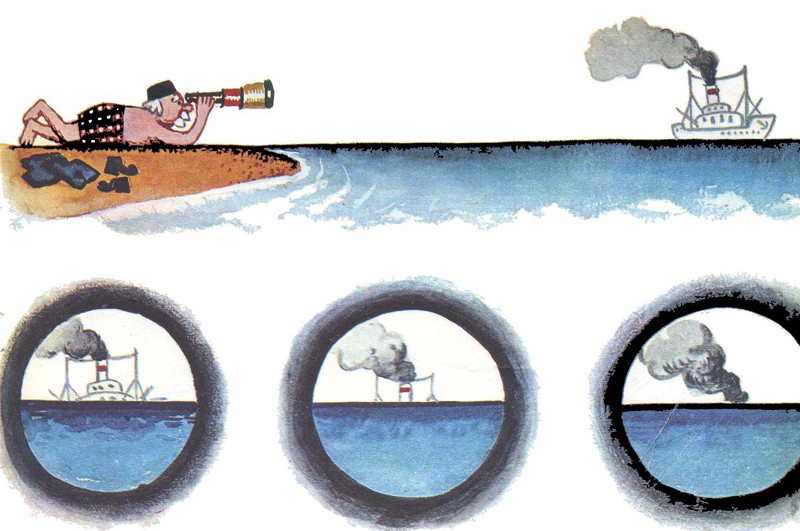
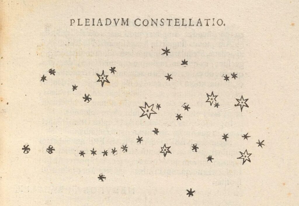
The star variable has the names of the stars as seen in the table above. Many of the names are of ancient and mythological origins, while some are modern. Most are of Arabic origin, while few are from Latin. Have a look at Star Lore of All Ages by William Olcott to know some of the mythologies associated with these names. Typically the alphabets after the star names indicate them being part of a stellar system, for example Alpha Centauri is a triple star system. The nomenclature is such that A represents the brightest member of the system, B the second brightest and so on. Also notice that some names have Greek pre-fixes, as in the case of of Alpha Centauri. This Greek letter scheme was introduced by Bayer in 1603 and is known as Bayer Designation. The Greek letters  denote the visual magnitude or brightness (we will come to the meaning of this next) of the stars in a given constellation. So Alpha Centuari would mean the brightest star in the Centaurus constellation. Before invention of the telescope the number of stars that are observable were limited by the limits of human visual magnitude which is about +6. With invention of telescope and their continuous evolution with increasing light gathering power, we discovered more and more stars. Galileo is the first one to view new stars and publish them in his Sidereal Messenger. He shows us that seen through the telescope, there are many more stars in the Pleiades constellation than can be seen via naked eyes (~+6 to max +7 with about 4200 stars possibly visible).

Soon, so many new stars were discovered that it was not possible to name them all. So coding of the names begun. The large telescopes which were constructed would do a sweep of the sky using big and powerful lenses and would create catalogue of stars. Some of the names in the data set indicate these data sets, for example HD denotes Henry Draper Catalogue.

Magnitudes of stars

Now let us look at the other three columns present us with observations of these stars. Let us understand what they mean. The second column represents magnitude of the stars. The stellar magnitude is of two types: apparent and absolute. The apparent magnitude is a measure of the brightness of the star and depends on its actual brightness, distance from us and any loss of the brightness due to intervening media. The magnitude scale was devised by Claudius Ptolemy in second century. The first magnitude stars were the brightest in the sky with sixth being the dimmest. The modern scale follows this classification and has made it mathematical. The scale is reverse logarithmic, meaning that lower the magnitude, brighter is the object. A magnitude difference of 1.0 corresponds to a brightness ratio of $ \sqrt[5]{100} $ or about 2.512. Now if you are wondering why the magnitude scale is logarithmic, the answer lies in the physiology of our visual system. As with the auditory system, our visual system is not linear but logarithmic. What this means is that if we perceive an object to be of double brightness of another object, then their actual brightness (as measured by a photometer) are about 2.5. This fact is encapsulated well in the Weber-Fechnar law. The apparent magnitude of the Sun is about -26.7, it is after all the brightest object in the sky for us. Venus, when it is brightest is about -4.9. The apparent magnitude of Neptune is +7.7 which explains why it was undiscovered till the invention of the telescope.

But looking at the table about the very first entry lists Sun’s magnitude as +4.8. This is because the dataset contains the absolute magnitude and not the apparent magnitude. Absolute magnitude is defined as “apparent magnitude that the object would have if it were viewed from a distance of exactly 10 parsecs (32.6 light-years), without dimming by interstellar matter and cosmic dust.” As we know, the brightness of an object is inversely proportional to square of the distance (inverse square law). Due to this fact very bright objects can appear very dim if they are very far away, and vice versa. Thus if we place the Sun at a distance of about 32.6 light years it will be not-so-bright and will be an “average” star with magnitude +4.8. The difference in these two magnitudes is -31.57 and this translates to huge brightness difference of 3.839 $\times$ 1012. And of course this  definition does not take into account the interstellar matter which further dims the stars. Thus to find the absolute magnitude of the stars we also need to know their distance. This is possible for some nearby stars for which the parallax has been detected. But for a vast majority of stars, the parallax is too small to be detected because they are too faraway. The distance measure parsec we saw earlier is defined on basis of parallax, one parsec is the distance at which 1 AU (astronomical unit: distance between Earth and Sun) subtends an angle of one arcsecond or 1/3600 of a degree.

Thus finding distance to the stars is crucial if we want to know their actual magnitudes. For finding the cosmic distances various techniques are used, we will not go into their details. But for our current purpose, we know that the stars dataset has absolute magnitudes of stars. The range of magnitudes in the dataset is

> range(stars$magnitude)
[1] -8 17

Thus stars in the dataset have a difference of 25 magnitudes, that is a brightness ratio of 105! Which are these brightest and dimmest stars? And how many stars of each magnitude are there in the data set? We can answer these type of questions with simple queries to our dataset. For starters let us find out the brightest and dimmest stars in the dataset. Each row in the dataset has an index, which is the first column in the table from RStudio above. Thus if we were to write:

> stars[1]

it will give us all the entries of the first column,

star
1 Sun
2 SiriusA
3 Canopus
4 Arcturus
5 AlphaCentauriA
6 Vega
7 Capella
8 Rigel
9 ProcyonA
10 Betelgeuse
...
...

But if we want only a single row, instead of a column, we have to tell that by keeping a , in the index 1. Thus for the first row we write

> stars[1,]
> star magnitude temp type
1 Sun 4.8 5840 G

Thus to find the brightest or dimmest star we will have to find its index and then we can find its name from the corresponding column. So how do we do that? For this we have functions which.max and which.min, we use them thus:

> which.max(stars$magnitude)
[1] 76

We feed this to the dataset and get

> stars[76,]
star magnitude temp type
76 G51-I5 17 2500 M

This can also be done in a single line

> stars[which.min(stars$magnitude), ]
star magnitude temp type
45 DeltaCanisMajoris -8 6100 F

Now let us check the distribution of these magnitudes. The simplest way to do this is to create a  histogram using the hist function.

hist(stars$magnitude)

This gives the following output

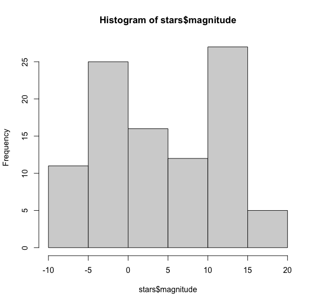
As we can see it has by default binned the magnitudes in bins of 5 units and the distribution here is bimodal with one peak between -5 and 0 and another peak between 10 and 15. We can tweak the width of the bars to get a much finer picture of the distribution. For this hist function has option to add breaks manually. We have used the seq function here ranging from -10 to 20 in steps of 1.

> hist(stars$magnitude, breaks = seq(-10, 20, by = 1))

And this gives us:

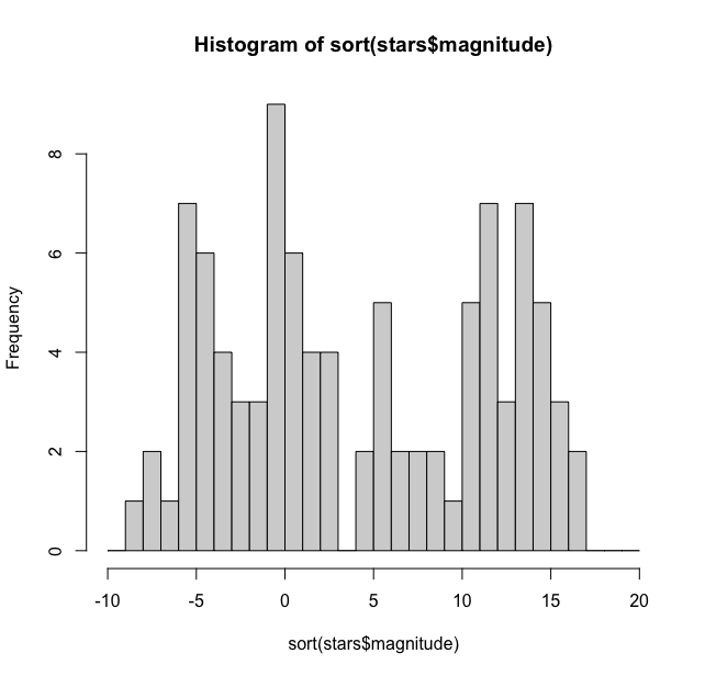
Thus we see that the maximum number of stars (9) are at -1 magnitude  and three magnitudes have one star each while +3 magnitude doesn’t have any stars. This histogram could be made more reader friendly if we can add the count on the bars. For this we need to get some coordinates and numbers. We first get the counts

mag_data <- hist(stars$magnitude, breaks = seq(-10,20, 1), plot = FALSE)

This will give us the actual number of counts

> [1] 0 1 2 1 7 6 4 3 3 9 6 4 4 0 2 5 2 2 2 1 5 7 3 7 5 3 2 0 0 0

Now to place them at the middle of the bars of histogram we need midpoints of the bars, we use mag_data$mids to find them and mag_data_counts for the count for labels.

> text(mag_data$mids, mag_data$counts, labels = mag_data$counts, pos = 3, cex = 0.8, col = "black")

To get the desired graph

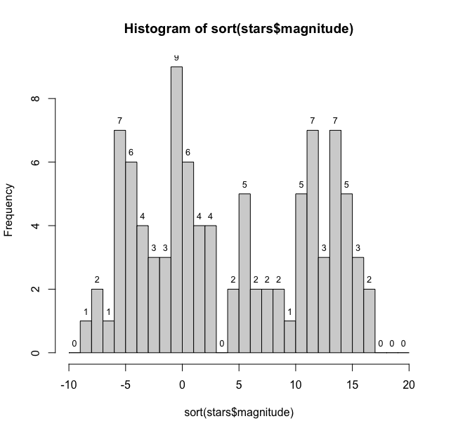
Thus we have a fairly large distribution of stellar magnitudes.

Now if we ask ourselves this question How many stars in this dataset are visible to the naked eye? What can we say? We know that limiting magnitude for naked eye is +6. So, a simple query should suffice:

count(stars %>% filter(magnitude <= 6))
n
1 57

(Here we have used the pipe function %>% to pass on data from one argument to another from the dplyr pacakge. This query shows that we have 57 stars which have magnitude less than or equal to 6. Hence these many should be visible… But wait it is the absolute magnitude that we have in this dataset, so this question itself cannot be answered unless we have the apparent magnitudes of the stars. Though computationally correct, this answer has no meaning as it is cannot be treated same as the one with apparent magnitude which we experience while watching the stars.

Temperature of Stars

The third column in the data set is the temp or the temperature. Now, at one point in the history of astronomy people believed that we would never be able to understand the structure or the content of the stars. But the invention of spectroscopy as a discipline and its application to astronomy made this possible. With the spectroscope applied to the end of the telescope (astronomical spectroscopy), we could now understand the composition of the stars, their speed and their temperature. The information for the composition came from the various emission and absorption lines in the spectra of the stars, which were then compared with similar lines produced in the laboratory by heating various elements. Helium was first discovered in this manner: first in the spectrum of the Sun and then in the laboratory. For detailed story of stellar spectroscopy one can see the book Astronomical Spectrographs and Their History by John Hearnshaw. Though an exact understanding of the origin of the spectral line came only after the advent of quantum mechanics in early part of 20th century.

But the spectrum also tells us about the surface temperature of the stars. How this is so? For this we need to invoke one of the fundamental ideas in physics: the blackbody radiation. Now if we find the intensity of radiation from a body at different wavelengths (or frequencies) we get a curve. This curve is typical and for different temperatures we get unique curves (they don’t intersect). Of course this is true for an ideal blackbody which is an idealized opaque, non-reflective body. Stellar spectrum is like that of an ideal blackbody,  this continuous spectrum is punctuated with absorption and emission lines as shown in the book cover above.

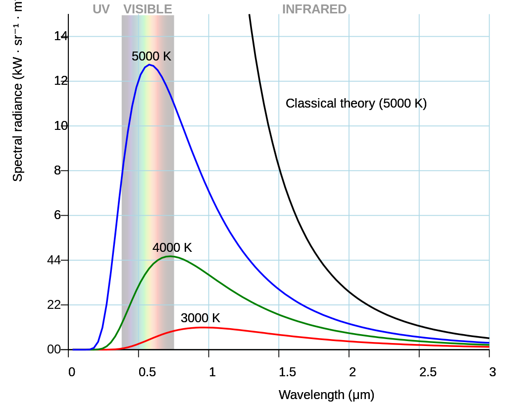
The frequency or wavelength at which the radiation has maximum intensity (brightness/luminosity) is related to the temperature of the body, typical curves are shown as above. Stars behave almost as ideal black bodies. Notice that as the temperature of the body increases the peak radiation wavelength increases (frequency is reduced) as shown in the diagram above. These relationships are given by the formula

$$
L = 4 \pi R^{2} \sigma T^{4}
$$

where $L$ is the luminosity, $R$ is the radius, $\sigma$ is Stephan’s constant and $T$ is the temperature. This equation tells us that $L$ is much more dependent on the $T$, so hotter stars would be more brighter.

It was failure of the classical ideas of radiation and thermodynamics to explain the nature of blackbody radiation that led to formulation of quantum mechanics by Max Planck in the form of Planck’s law for quantisation of energy. For a detailed look at the history of this path breaking episode in history of science one of the classics is Thomas Kuhn’s Black-Body Theory and the Quantum Discontinuity, 1894—1912.

That is to say hotter bodies have shorter peak frequencies. In other words, blue stars are hotter than the red ones. (Our hot and cold symbolic colours on the plumbing peripherals needs to change: we have it completely wrong!) Thus the spectrum of the stars gives as its absolute temperature, along with all other information that we can obtain from the stars. The spectrum is our only source of information for stars. This is what is represented in the third column of our data. For our dataset the range of stellar temperatures we have a wide range of temperatures.

range(stars$temp)
[1] 2500 33600

Let us explore this column a bit. If we plot a histogram with default options we get:

> hist(stars$temp)

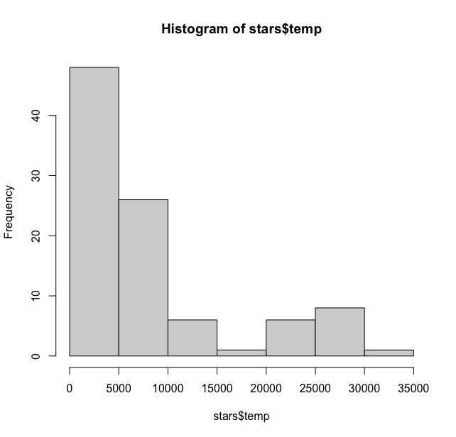
This is showing maximum stars have a temperature below 10000. We can bin at 1000 and add labels to get a much better sense. Which star has 0 temperature??

hist(stars$temp, breaks = seq(0,35000, 1000))
> temp_data <- hist(stars$temp, breaks = seq(0,35000, 1000), plot = FALSE)
> text(temp_data$mids, temp_data$counts, labels = temp_data$counts, pos = 3, cex = 0.8, col = "black")

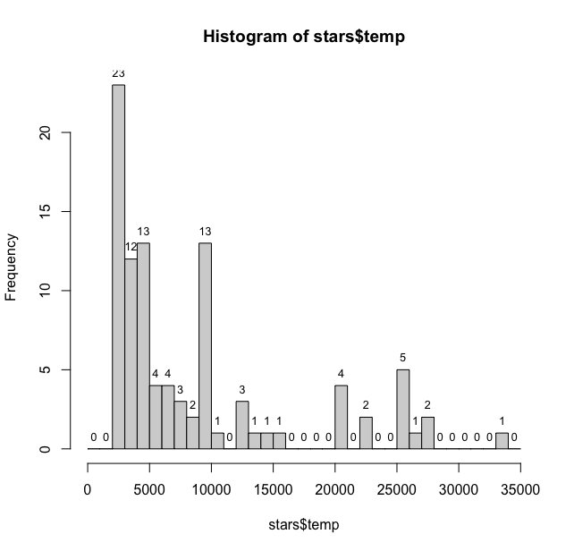
This plot gives us much better sense of the distribution of stellar temperatures. With most of the temperatures being in 2000-3000 degrees Kelvin range. The table() function also provides useful information about distribution of temperatures in the column.

> table(stars$temp)

2500 2670 2800 2940 3070 3200 3340 3480 3750 3870 4130 4590
1 10 7 5 1 3 4 1 1 2 3 3
4730 4900 4950 5150 5840 6100 6580 6600 7400 7700 8060 9060
1 5 1 2 2 2 1 1 2 1 2 1
9300 9340 9620 9700 9900 10000 11000 12140 12400 13000 13260 14800
1 2 3 1 4 1 1 1 1 1 1 1
15550 20500 23000 25500 26950 28000 33600
1 4 2 5 1 2 1

While the summary() function provides the basic statistics:

> summary(stars$temp)
Min. 1st Qu. Median Mean 3rd Qu. Max.
2500 3168 5050 8752 9900 33600

Type of Stars

The fourth and final column of our data is type. This category of data is again based on the spectral data of stars and is type of spectral classification of stars. “The spectral class of a star is a short code primarily summarizing the ionization state, giving an objective measure of the photosphere’s temperature. ” The categories of the type of stars and their physical properties are summarised in the table below. The type of stars and their temperature is related, with “O” type stars being the hottest, while “M” type stars are the coolest. The Sun is an average “G” type star.

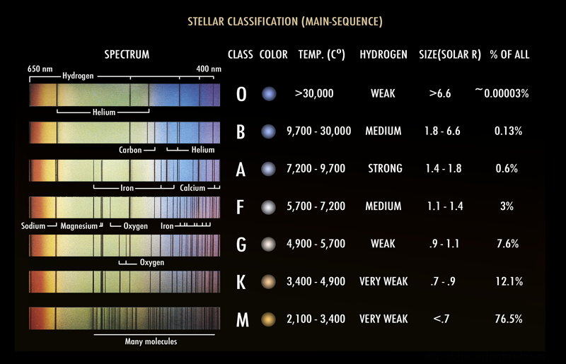
There are several mnemonics that can help one remember the ordering of the stars in this classification. One that I still remember from by Astrophysics class is Oh Be A Fine Girl/Guy Kiss Me Right Now. Also notice that this “type” classification is also related to size of the stars in terms of solar radius.

In our dataset, we can see what type of stars we have by

> stars$type
[1] "G" "A" "F" "K" "G" "A" "G" "B" "F" "M" "B" "B" "A" "K"
[15] "B" "M" "A" "K" "A" "B" "B" "B" "B" "B" "B" "A" "M" "B"
[29] "K" "B" "A" "B" "B" "F" "O" "K" "A" "B" "B" "F" "K" "B"
[43] "B" "K" "F" "A" "A" "F" "B" "A" "M" "K" "M" "M" "M" "M"
[57] "M" "A" "DA" "M" "M" "K" "M" "M" "M" "M" "K" "K" "K" "M"
[71] "M" "G" "F" "DF" "M" "M" "M" "M" "K" "M" "M" "M" "M" "M"
[85] "M" "DB" "M" "M" "A" "M" "K" "DA" "M" "K" "K" "M"

Our Sun is G-type star in this classification (first entry). If we use the table() function on this column we get the frequency of each type of star in the dataset.

> table(stars$type)

A B DA DB DF F G K M O
13 19 2 1 1 7 4 16 32 1

And to see a barplot of this table we will use ggplot2() package. Load the package using library using library(ggplot2) and then

> stars %>% ggplot(aes(type)) + geom_bar() + geom_text(stat = "count", aes(label = after_stat(count)), vjust = -0.5, size = 4)

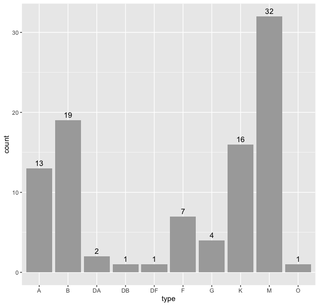
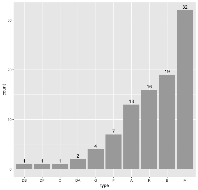
Thus we see that “M” type stars are the maximum in our dataset. But we can do better, we can sort this data according the frequency of the types. For this we use the code:

> type_count <- table(stars$type) > # count the frequencies
> sorted_type <- names(sort(type_count)) > # sort them
> stars$type <- factor(stars$type, levels = sorted_type) > # reorder them with levels and plot them
> stars %>% ggplot(aes(type)) + geom_bar(fill = "darkgray") + geom_text(stat = "count", aes(label = after_stat(count)), vjust = -0.5, size = 4)

And we get

To plot HR Diagram

Now, given my training in astronomy and astrophysics, the first reaction that came to my mind after seeing this data was this is the data for the HR Diagram! The HR diagram presents us with the fundamental relationship of types and temperature of stars. This was an crucial step in understanding stellar evolution. The intials HR stand for the two astronomers who independently found this relationship: The diagram was created independently in 1911 by Ejnar Hertzsprung and by Henry Norris Russell in 1913.

By early part of 20th century several star catalogues had been around, but nothing stellar evolution or structure was known. The stellar spectrographs revealed what elements were present in the stars, but the energy source of the stars was still an unresolved question. Classical physics had no answer to this fundamental question about how stars were able to create so much energy (for example, see Stars A Very Short Introduction by James Kaler on the idea that charcoal powers the Sun by Lord Kelvin). Added to this was the age of the stars, from geological data and idea of geological deep time, the Sun was estimated to be 4 billion years old as was the Earth. So stars had been producing so much energy for such a long time! But that is not the point of this post, the HR diagram definitely helped the astronomers think about the idea that stars might not be static but evolve in time. The International Astronomical Union conducted a special symposium titled The HR Diagram in 1977. The proceedings of the symposium have several articles of interest on the history of creation and interpretation of the HR Diagram.

I think it was but natural that astronomers tried to find correlations between various properties of thousands of stars in these catalogues. And when they did they find a (co-)relationship between them. The HR diagram exists in many versions, but the basic idea is to plot the absolute magnitude and temperature (or colour index). Let us plot these two  to see the co-relation, for this we again use the ggplot2() pacakge and its scatterplot function geom_point().

> stars %>% ggplot(aes(temp, magnitude)) + geom_point()

This gives us the basic plot of HR diagram.

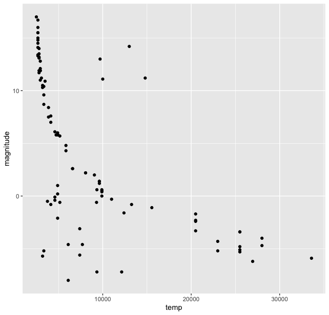
Immediately we can see that the stars are not randomly scattered on this plot, but are grouped in clusters. And most of them lie in a “band”. Though there are outliers at the lower temperature and magnitude range and high magnitude and temperature around 10-15 thousand range. We see that most stars lie in a band which is called the “Main Sequence”. We can try to fit a function here in this plot using some options in the ggplot() library, we use geom_smooth() function for this and get:

stars %>% ggplot(aes(temp, magnitude)) + geom_point() + geom_smooth( se = FALSE, color = “red”)

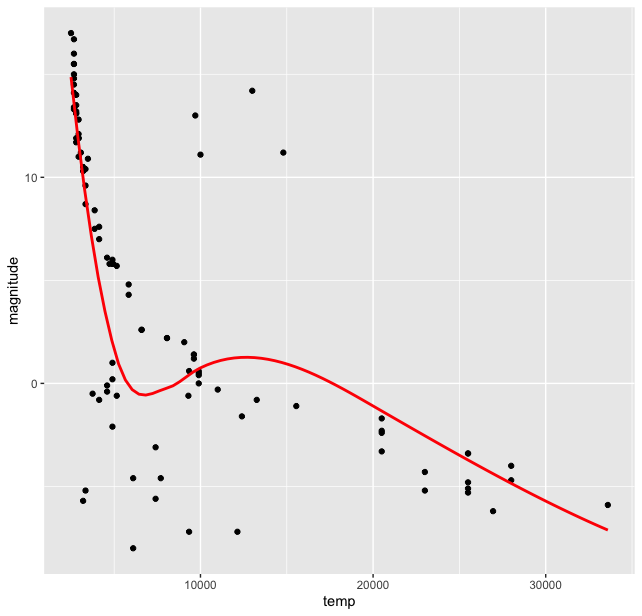
Of course this smooth curve is a very crude (perhaps wrong?) approximation of the data, but it certainly points us towards some sort of correlation between the two quantities for most of the stars. But wait, we have another categorical variable in our dataset, the type of stars. How are the different types of stars distributed on this curve? For this we introduce type variable in the aesthetics argument of ggplot() to colour the stars on our plot according to this category:

> stars %>% ggplot(aes(temp, magnitude, color = type)) + geom_smooth( se = FALSE, color = "red") + geom_point()

This produces the plot

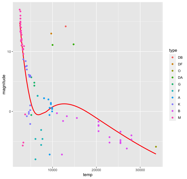
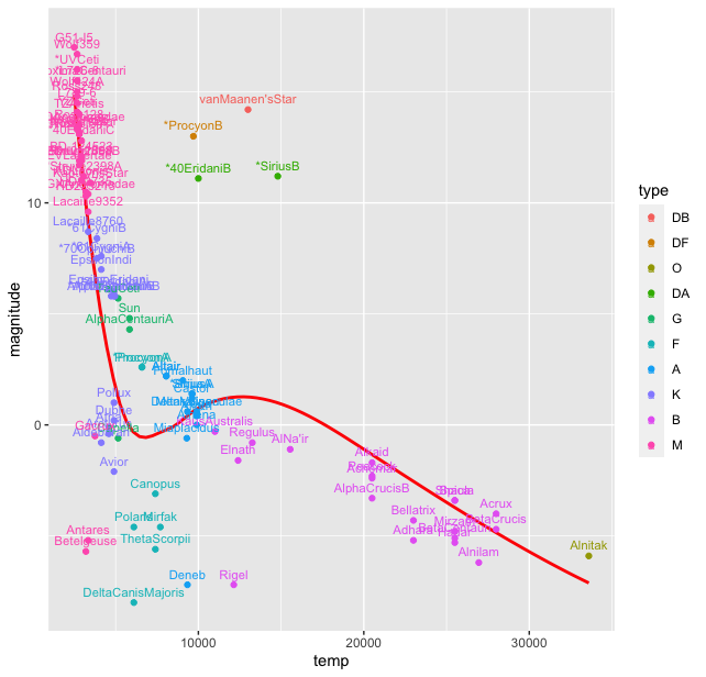
Thus we see there is a grouping of stars by the type. Of course the colours in the palette here are not the true representatives of the star colours. The HR diagram was first published around 1911-13, when quantum mechanics was in its nascent stages. The ideas of Rutherford’s model were still extant and was just out. The fact that this diagram indicated a relationship between the magnitude and temperature, led to thinking about stellar structure itself and its ways of producing energy with fundamentally new ideas about matter and energy from quantum mechanics and their transformation from relativistic physics. But that is a story in future. For now, let us come to our HR diagram. From the dataset we have one more variable, the star name which could be used in this plot. We can name all the stars in the plot (there are only 96). For this we use the geom_text() function in ggplot()

> stars %>% ggplot(aes(temp, magnitude, color = type), label = star) + geom_smooth( se = FALSE, color = "red") + geom_point() + geom_text((aes( label = star)), nudge_y = 0.5, size = 3)

This produces a rather messy plot, where most of the starnames are on top of each other and not readable:

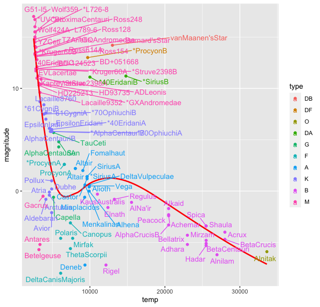
To overcome this clutter we use another package ggrepel() with the following code:

> stars %>% ggplot(aes(temp, magnitude, color = type), label = star) + geom_smooth( se = FALSE, color = "red") + geom_text_repel(aes(label = star))

This produces the plot with the warning "Warning message: ggrepel: 13 unlabeled data points (too many overlaps). Consider increasing max.overlaps ". To overcome this we increase the max.overlaps to 50.

> stars %>% ggplot(aes(temp, magnitude, color = type), label = star) + geom_point() + geom_smooth( se = FALSE, color = "red") + geom_text_repel(aes(label = star), max.overlaps = 50)


This still appears cluttered a bit, scaling the plot while exporting gives this plot, though one would need to zoom in to read the labels.

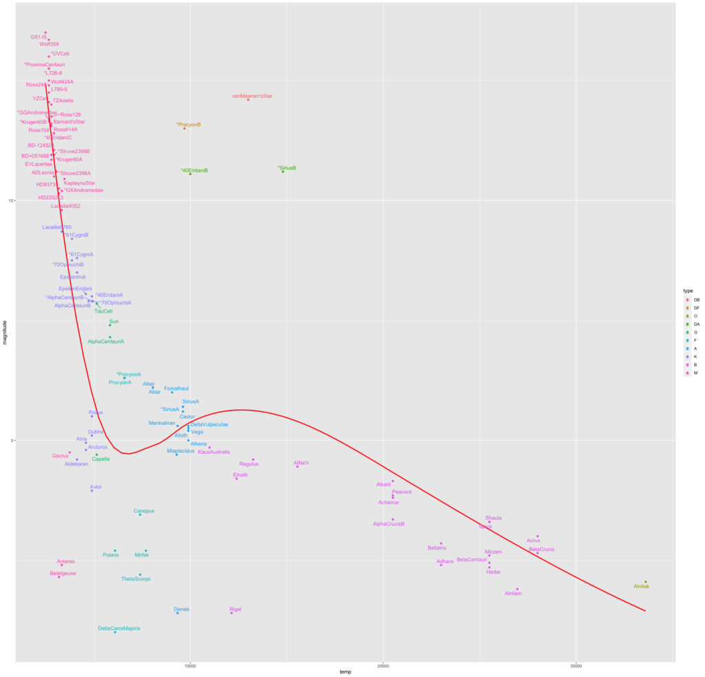
Of course with a different data set, with larger number and type of stars we would see slightly different clustering, but the general pattern is the same.

We thus see that starting from the basic data wrangling we can generate one of the most important diagrams in astrophysics. I learned a lot of R in the process of creating this diagram. Next task is to

How big is the shadow of the Earth?


The Sun is our ultimate light source on Earth. The side of the Earth facing the Sun is bathed in sunlight, due to our rotation this side changes continuously. The side which faces the Sun has the day, and the other side is the night, in the shadow of the entire Earth. The sun being an extended source (and not a point source), the Earth’s shadow had both umbra and penumbra. Umbra is the region where no light falls, while penumbra is a region where some light falls. In case of an extended source like the Sun, this would mean that light from some part of the Sun does fall in the penumbra.  Occasionally, when the Moon falls in this shadow we get the lunar eclipse. Sometimes it is total lunar eclipse, while many other times it is partial lunar eclipse. Total lunar eclipse occurs when the Moon falls in the umbra, while partial one occurs when it is in penumbra. On the other hand, when the Moon is between the Earth and the Sun, we get a solar eclipse. The places where the umbra of the Moon’s shadow falls, we get total solar eclipse, which is a narrow path on the surface of the Earth, and places where the penumbra falls a partial solar eclipse is visible. But how big is this shadow? How long is it? How big is the umbra and how big is the penumbra? We will do some rough calculations, to estimate these answers and some more to understand the phenomena of eclipses.

We will start with a reasonable assumption that both the Sun and the Earth as spheres. The radii of the Sun, the Earth and the Moon, and the respective distances between them are known. The Sun-Earth-Moon system being a dynamic one, the distances change depending on the configurations, but we can assume average distances for our purpose.

[The image above is interactive, move the points to see the changes. This construction is not to scale!. The simulation was created with Cinderella ]


The diameter of the Earth is approximately 12,742 kilometers, and the diameter of the Sun is about 1,391,000 kilometers, hence the ratio is about 109, while the distance between the Sun and the Earth is about 149 million kilometers. A couple of illustrations depicting it on the correct scale.


The Sun’s (with center A) diameter is represented by DF, while EG represents Earth’s (with center C) diameter. We connect the centers of Earth and Sun. The umbra will be limited in extent in the cone with base EG and height HC, while the penumbra is infinite in extent expanding from EG to infinity. The region from umbra to penumbra changes in intensity gradually. If we take a projection of the system on a plane bisecting the spheres, we get two similar triangles HDF and HEG. We have made an assumption that our properties of similar triangles from Euclidean geometry are valid here.

In the schematic diagram above (not to scale) the umbra of the Earth terminates at point H. Point H is the point which when extended gives tangents to both the circles. (How do we find a point which gives tangents to both the circles? Is this point unique?). Now by simple ratio of similar triangles, we get

$$
\frac{DF}{EG} = \frac{HA}{HC}  = \frac{HC+AC}{HC}
$$

Therefore,

$$
HC = \frac{AC}{DF/EG -1}
$$

Now, $DF/EG = 109$, and $AC$ = 149 million km,  substituting the values we get the length of the umbra $HC \approx$  1.37 million km. The Moon, which is at an average distance of 384,400 kilometers,  sometimes falls in this umbra, we get a total lunar eclipse. The composite image of different phases of a total lunar eclipse below depicts this beautifully. One can “see” the round shape of Earth’s umbra in the central three images of the Moon (red coloured) when it is completely in the umbra of the Earth (Why is it red?).

When only a part of umbra falls on the moon we get a partial lunar eclipse as shown below. Only a part of Earth’s umbra is on the Moon.

So if the moon was a bit further away, lets say at 500,000 km, we would not get a total solar eclipse. Due to a tilt in Moon’s orbit not every new moon is an eclipse meaning that the Moon is outside both the umbra and the penumbra.

The observations of the lunar eclipse can also help us estimate the diameter of the Moon.

Similar principle applies (though the numbers change) for solar eclipses, when the Moon is between the Earth and the Sun. In case of the Moon, ratio of diameter of the Sun and the Moon is about 400. With the distance between them approximately equal to the distance between Earth and the Sun. Hence the length of the umbra using the above formula is 0.37 million km or about 370,000 km. This makes the total eclipse visible on a small region of Earth and is not extended, even the penumbra is not large (How wide is the umbra and the penumbra of the moon on the surface of the Earth?).

When only penumbra is falling on a given region, we get the partial solar eclipse.

You can explore when solar eclipse will occur in your area (or has occurred) using the Solar Eclipse Explorer.

This is how the umbra of the Moon looks like from space.

And same thing would happen to a globe held in sunlight, its shadow would be given by the same ratio.

Thus we see that the numbers are almost matched to give us total solar eclipse, sometimes when the moon is a bit further away we may also get what is called the annular solar eclipse, in which the Sun is not covered completely by the Moon. Though the total lunar eclipses are relatively common (average twice a year) as compared to total solar eclipses (once 18 months to 2 years). Another coincidence is that the angular diameters of the Moon and the Sun are almost matched in the sky, both are about half a degree (distance/diameter ratio is about 1/110). Combined with the ratio of distances we are fortunate to get total solar eclipses.

Seeing and experiencing a total solar eclipse is an overwhelming experience even when we have an understanding about why and how it happens. More so in the past, when the Sun considered a god, went out in broad daylight. This was considered (and is still considered by many) as a bad omen. But how did the ancient people understand eclipses?  There is a certain periodicity in the eclipses, which can be found out by collecting large number of observations and finding patterns in them. This was done by ancient Babylonians, who had continuous data about eclipses from several centuries. Of course sometimes the eclipse will happen in some other part of the Earth and not be visible in the given region, still it could be predicted.   To be able to predict eclipses was a great power, and people who could do that became the priestly class. But the Babylonians did not have a model to explain such observations. Next stage that came up was in ancient Greece where models were developed to explain (and predict) the observations. This continues to our present age.

The discussion we have had applies in the case when the light source (in this case the Sun) is larger than the opaque object (in this case the Earth). If the the light source is smaller than the object what will happen to the umbra? It turns out that the umbra is infinite in extent. You see this effect when you get your hand close to a flame of candle and the shadow of your hand becomes ridiculously large! See what happens in the interactive simulation above.

References

James Southhall Mirrors, Prisms and Lenses (1918) Macmillan Company

Eric Rogers Physics for the Inquiring Mind (1969) Princeton


EM Spectrum in Astronomy

EM Spectrum in Astronomy from Astrobites

I created a mindmap from the information above

  • Radio
    λ > 1 mm
    ν < 300 GHz

    • Objects
      • AGN JEts
      • Supernovae
      • Tidal Disruption Events
      • H II regions
      • Gamma ray bursts
      • Radio Galaxies
    • Processes
      • Synchrotron radiation
      • Free-free radiation
    • Observation
      • Ground based
    • Telescopes
      • Green Bank Telescope (GBT)
      • Five-hundred-meter Aperture Spherical Telescope (FAST)
      • Very Large Array (VLA)
      • Square Kilometer Array (SKA)
      • Low-Frequency Array (LoFAR),
      • Giant Meterwave Radio Telescope (GMRT)
  • Microwave/Sub-mm
    λ ~ 300 μm to 1 mm
    ν ~ 1 THz to 300 GHz

    • Objects
      • CMB
      • High energy phenomena
        • Relativistic jets
        • Cold dust
        • Cold gas
        • Galaxies at high z
    • Processes
      • Thermal (blackbody radiation)
    • Observation
      • Space
      • Ground
    • Telescopes
      • Space
        • Cosmic Background Explorer (COBE)
        • Wilkinson Microwave Anisotropy Probe (WMAP)
        • Planck
      • Ground
        • Submillimeter Array (SMA
        • Atacama Large Millimeter/submillimeter Array (ALMA).
  • Infrared
    λ ~ 300 μm to 2.5 μm
    ν ~ 1 THz to 120 THz

    • Far-Infrared
      λ ~ 15 μm to 300 μm
      ν ~ 20 THz 1 THz

      • Objects
        • Cool dust
        • Cool gas
        • star forming galaxies
        • young stellar objects
          • proto-stars
          • pre-main sequence stars
      • Processes
        • Thermal (Blackbody radiation)
      • Observation
        • Space
      • Telescopes
        • Infrared Astronomical Satellite (IRAS)
        • Infrared Space Observatory (ISO)
        • Herschel
    • Mid-Infrared
      λ ~ 2.5 μm to 15 μm
      ν ~ 120 THz 20 THz

      • Objects
        • Cosmic dust
          • surrounding young stars
          • protoplanetary disks
          • zodiacal dust
        • Solar system objects
          • planets
          • comets
          • asteroids
      • Processes
        • Thermal (Blackbody Radiation)
      • Observation
        • Space
        • Ground
      • Telescopes
        • Ground
          • Infrared Telescope Facility (IRTF)
          • United Kingdom Infrared Telescope (UKIRT)
        • Space
          • James Webb Space Telescope
          • Wide-field Infrared Survey Explorer (WISE)
          • Spitzer
    • Near-Infrared
      λ ~ 0.8 μm to 2.5 μm
      ν ~ 380 THz 120 THz

      • Objects
        • M-dwarfs
        • Cool stars
        • Low-mass stars
        • Galaxies
      • Processes
        • Thermal (Blackbody Radiation)
      • Observation
        • Space
        • Ground
      • Telescopes
        • Ground
          • 2MASS survey
          • Infrared Telescope Facility (IRTF)
          • United Kingdom Infrared Telescope (UKIRT)
          • Visible and Infrared Survey Telescope for Astronomy (VISTA)
        • Space
          • James Webb Space Telescope
  • Optical
    λ ~ 350 nm to 800 nm
    ν ~ 860 THz 380 THz

    • Objects
      • Ionized gases
      • Stars
      • Galaxies
    • Processes
      • Black Body Radiation (Thermal)
      • Non-thermal
    • Observation
      • Both Ground and Space
    • Telescopes
      • Ground
        • W.M. Keck telescopes
        • Very Large Telescopes
        • Southern African Large Telescope (SALT)
      • Space
        • Hubble Space Telescope
        • Gaia
        • Kepler
        • Transiting Exoplanet Survey Satellite (TESS).
  • Ultra-violet
    λ ~ 10 nm to 350 nm
    ν ~ 3e16 Hz to 860 Hz
    E ~ 120 eV to 3.5 eV

    • Objects
      • Thermal
        • O Stars
        • B Stars
        • white dwarfs
      • Non-thermal
        • AGN (continuous emission)
    • Processes
      • Blackbody radiation (thermal radiation)
      • Non-thermal sources
    • Observation
      • Ground (longest)
      • Space
    • Telescopes
      • AstroSAT (2015)
      • Galaxy Evolution Explorer (GALEX) (2003)
      • Hubble Space Telescope (1990)
      • Neil Gehrels Swift Observatory (2004)
  • X-Ray
    λ ~ 10 pm to 10 nm
    ν ~ 3e19 Hz to 3e16 Hz
    E ~ 120 keV to 0.12 keV

    • Objects
      • X-Ray binaries
      • AGN
      • Neutron stars
    • Processes
      • Thermal Emission
      • Free-Free emission
      • Accretion
    • Observation
      • From Space
    • Telescopes
      • Uhuru (1973)
      • Einstein (1978-81)
      • ROSAT (1999)
      • Chandra (1999)
      • XMM-Newton (1999)
      • NuSTAR (2012)
      • eROSITA (2019)
    • Gamma-Ray
      λ < 10 pm
      ν > 3e19 Hz
      E > 120 keV

      • Objects
        • AGN with Relativistic Jets
        • Gamma Ray Binaries
        • Gamma Ray Bursts
      • Processes
        • Gamma Decay
        • Pair-Annihilation
        • Shock Waves
        • Inverse-Compton Scattering
      • Observation
        • From Space
      • Telescopes
        • Compton Gamma-ray Observatory (1991)
        • International Gamma-Ray Astrophysics Laboratory (INTEGRAL) (2002)
        • Fermi (2008)

//mm2html.xsl FreeplaneVersion:freeplane 1.2.0

Interesting LaTeX Packages – Drawing the Solar System

Many times we need to quickly illustrate the solar system or the planets. Usually we use photos to illustrate the planets. But sometimes the photos can be an over kill. Also to draw the entire solar system is a typical and can be used for illustrative purposes. Though most of the illustrations of the solar system in the school and other text books are horribly out of scale, (with no indication that the figure is not to scale!). For example,  look at the illustration in the Class 6 Science Textbook from NCERT.

A good visualisation will always present a scale, and/or indicate whether the visualisation is to the scale or not. Though in the visualisation above the distances are given, they are not to scale.


Coming back to the topic of our post, a simple way to draw solar system diagram in latex is to use the PStricks package solarsystem. The package can create “Position of the visible planets, projected on the plane of the ecliptic” at a given time and date. This feature might be useful sometimes.

From the package manual:

As we can not represent all the planets in the real proportions, only Mercury, Venus, Earth and Mars are the proportions of the orbits and their relative sizes observed. Saturn and Jupiter are in the right direction, but obviously not at the right distance.
The orbits are shown in solid lines for the portion above the ecliptic and dashed for the portion located below.

The use of the command is very simple, just specify the date of observation with the following parameters, for example:
\SolarSystem[Day=31,Month=12,Year=2020,Hour=23,Minute=59,Second=59]
By default, if no parameter is specified, \SolarSystem gives the configuration day 0 hours to compile.

The resulting output for the above code:

The output also provides the longitude and latitude of the planets at the time given.

Another package that is useful to create free standing planets is the tikz-planets package which we will see next.

The Astronomers

Looking at this vast natural drama from their observation posts on the minute planet Earth as it revolves around the insignificant star called the sun, a handful of astronomers seek to gain an understanding of the cosmos. Using instruments constructed from materials found on their planet, they follow the activities in space from their observatories and launch rocket-borne telescopes from Earth. Some people confuse them with astrologers, but astronomers reject all such notions of kinship; others look up to them because their thoughts and ideas move in realms beyond the imagination of those of us engaged in everyday activities. Their work brings them a step closer to creation, at least to the creation of the uninhabited world, but they are sober scientists who do not attempt to adduce ethical norms from the phenomena they observe. Their involvement with cosmic matters does not make them better human beings. They are not motivated solely by a dedication to greater knowledge. As is true of other segments of human society, thoughts of competition and career advancement enter into their calculations; quite a few discoveries grew out of just such considerations. Yet this is not to deny, as we shall learn, that we find among them a passion for knowledge and much friendly cooperation. The fruit of their research is the work of human beings and as such is often imperfect, even erroneous. But despite setbacks the course of the science of astronomy, beginning with the Babylonians and culminating in modern astrophysics, has led ever forward.

Rudolph Kippenhahn, 100 Billion Suns p. 6-7

Book Review: Pendulum: Léon Foucault and the Triumph of Science by Amir D. Aczel

The book traces Leon Foucault’s ingenious approach to solving the problem of providing a terrestrial proof of rotation of the Earth. The pendulum he devised oscillates in a constant plane, and if properly engineered (as he did) can actually show the rotation of the Earth. The demonstration is one the most visually impressive scientific experiments. Also, Foucault gave prediction, an equation which would tell us how the pendulum will behave at different parts of the Earth. The pure mathematicians and physicists alike were taken aback at this simple yet powerful demonstration of the proof which eluded some of the most brilliant minds, which includes likes of Galileo and Newton. Rushed mathematical proofs were generated, some of the mathematicians earlier had claimed that no such movement was possible. That being said, Foucault was seen as an outsider by the elite French Academy due to his lack of training and degree. Yet he was good in designign things and making connections to science. This was presented to the public in 1851, and the very next year in 1852 he created another proof for rotation of the Earth. This was done by him inventing the gyroscope.. Gyroscope now plays immense role in navigation and other technologies. Yet he was denied membership to the Academy, only due to interest of the Emperor Napolean III in his work in 1864. The pendulum is his most famous work, but other works are also of fundamental significance.

  • He was first person to do photomicrography using Daguerreotype
  • Accurate measurment of speed of light using rotating mirrors –
  • Devised carbon arc electric lamp for lighting of micrcoscope
  • One of the first to Daguerreotype the Sun
  • Designed the tracking systems used in telescopes
  • also designed many motors, regulators to control electrical devices

There are a couple of places in the book where Aczel seems to be confused, at one point he states parallax as a proof for rotation of Earth around its axis, whearas it is more of a proof of Earths motion around the Sun. At another place he states that steel was invented in 1800s which perhaps he means to say that it was introduced in the west at the time. Apart from this the parallels between the rise of Napoleon III, a Nephew of Napolean, to form the second Empire in France and Foucault’s own struggle for recognition of his work and worth is brought out nicely.

Rotating Earth: the proofs or significance of Leon Foucault’s pendulum – Part 1

rotating-earth
In an earlier post, we had discussed proofs of the round shape of the Earth. This included some ancient and some modern proofs. There was, in general, a consensus that the shape of the Earth was spherical and not flat and the proofs were given since the time of ancient Greeks. Only in the middle ages, there seems to have been some doubt regarding the shape of the Earth. But amongst the learned people, there was never a doubt about the shape of the Earth. Counter-intuitive it may seem when you look at the near horizon, it is not that counter-intuitive. We can find direct proofs about it by looking around and observing keenly.
But the rotation of Earth proved to be a more difficult beast to tame and is highly counter-intuitive. Your daily experience does not tell you the Earth is rotating, rather intuition tells you that it is fixed and stationary. Though the idea of a moving Earth is not new, the general acceptance of the idea took a very long time. And even almost 350 years after Copernicus’ heliocentric model was accepted, a direct proof of Earth’s rotation was lacking. And this absence of definitive proof was not due to a lack of trying. Some of the greatest minds in science, mathematics and astronomy worked on this problem since Copernicus but were unable to solve it. This included likes of Galileo, Newton, Descartes, and host of incredibly talented mathematicians since the scientific revolution. Until Leon Foucaultin the mid-1800s provided not one but two direct proofs of the rotation of the Earth. In this series of posts, we will see how this happened.
When we say the movement of the Earth, we also have to distinguish between two motions that it has: first its motion about its orbit around the Sun, and second its rotational motion about its own axis. So what possible observational proofs or direct evidence will allow us to detect the two motions? In this post, we will explore how our ideas regarding these two motions of the Earth evolved over time and what type of proofs were given for and against it.

Even more, there was a simple geometrical fact directly opposed to the Earth’s annual motion around the Sun and there was nothing that could directly prove its diurnal rotation. (Mikhailov, 1975)

Let us consider the two components of Earth’s motion. The first is the movement around the Sun along the orbit. The simplest proof for this component of Earth’s motion is from the parallax that we can observe for distant stars. Parallax is the relative change in position of objects when they are viewed from different locations. The simplest example of this can be seen with our own eyes.
Straighten your hand, and hold your thumb out. Observe the thumb with both the eyes open. You will see your thumb at a specific location with respect to the background objects. Now close your left eye, and look at how the position of the thumb has changed with respect to the background objects. Now open the right eye, and close the left one. What we will see is a shift in the background of the thumb. This shift is related by simple geometry to the distance between our eyes, called the baseline in astronomical parlance. Thus even a distance of the order of a few centimetres causes parallax, then if it is assumed that Earth is moving around the Sun, it should definitely cause an observable parallax in the fixed stars. And this was precisely one of the major roadblock

Earth moving around an orbit raised mechanical objections that seemed even more serious in later ages; and it raised a great astronomical difficulty immediately. If the Earth moves in a vast orbit, the pattern of fixed stars should show parallax changes during the year. (Rogers, 1960)

The history of cosmic theories … may without exaggeration be called a history of collective obsessions and controlled schizophrenias.
– Arthur Koestler, The Sleepwalkers

Though it is widely believed that Copernicus was the first to suggest a moving Earth, it is not the case. One of the earliest proponents of the rotating Earth was a Greek philosopher named Aristarchus. One of the books by Heath on Aristarchus is indeed titled Copernicus of Antiquity (Aristarchus of Samos). A longer version of the book is Aristarchus of Samos: The Ancient Copernicus. In his model of the cosmos, Aristarchus imagined the Sun at the centre and the Earth and other planets revolving around it. At the time it was proposed, it was not received well. There were philosophical and scientific reasons for rejecting the model.

aristarchus-01
Aristarchus’s model of the heliocentric Universe

First, let us look at the philosophical reasons. In ancient Greek cosmology, there was a clear and insurmountable distinction between the celestial and the terrestrial. The celestial order and bodies were believed to be perfect, as opposed to the imperfect terrestrial. After watching and recording the uninterrupted waltz of the sky over many millennia, it was believed that the heavens were unchangeable and perfect. The observations revealed that there are two types of “stars”. First the so-called “fixed stars” do not change their positions relative to each other. That is to say, their angular separation remains the same. They move together as a group across the sky. Imagination coupled with a group of stars led to the conceiving of constellations. Different civilizations imagined different heroes, animals, objects in the sky. They formed stories about the constellations. These became entwined with cultures and their myths.
telescope_0013
The second type of stars did change their positions with respect to other “fixed stars”. That is to say, they changed their angular distances with “fixed stars”. These stars, the planets, came to be called as “wandering stars” as opposed to the “fixed stars”.

Ancient Greeks called these lights πλάνητες ἀστέρες (planētes asteres, “wandering stars”) or simply πλανῆται (planētai, “wanderers”),from which today’s word “planet” was derived.
Planet

So how does one make sense of these observations? For the fixed stars, the solution is simple and elegant. One observes the set of stars rising from the east and setting to the west. And this set of stars changes across the year (which can be evidenced by changing seasons around us). And this change was found to be cyclical. Year after year, with observations spanning centuries, we found that the stars seem to be embedded on inside of a sphere, and this sphere rotates at a constant speed. This “model” explains the observed phenomena of fixed stars very well.
The unchanging nature of this cyclical process observed, as opposed to the chaotic nature on Earth, perhaps led to the idea that celestial phenomena are perfect. Also, the religious notion of associating the heavens with gods, perhaps added to them being perfect. So, in the case of perfect unchanging heavens, the speeds of celestial bodies, as evidenced by observing the celestial sphere consisting of “fixed stars” was also to be constant. And since celestial objects were considered as perfect, the two geometrical objects that were regarded as perfect the sphere and the circle were included in the scheme of heavens. To explain the observation of motion of stars through the sky, their rising from the east and setting to the west, it was hypothesized that the stars are embedded on the inside of a sphere, and this sphere rotates at a constant speed. We being fixed on the Earth, observe this rotating sphere as the rising and setting of stars. This model of the world works perfectly and formed the template for explaining the “wandering stars” also.
These two ideas, namely celestial objects placed on a circle/sphere rotating with constant speed, formed the philosophical basis of Greek cosmology which would dominate the Western world for nearly two thousand years. And why would one consider the Earth to be stationary? This is perhaps because the idea is highly counter-intuitive. All our experience tells us that the Earth is stationary. The metaphors that we use like rock-solid refer to an idea of immovable and rigid Earth. Even speculating about movement of Earth, there is no need for something that is so obviously not there. But as the history of science shows us, most of the scientific ideas, with a few exceptions, are highly counter-intuitive. And that the Earth seems to move and rotate is one of the most counter-intuitive thing that we experience in nature.
The celestial observations were correlated with happenings on the Earth. One could, for example, predict seasons as per the rising of certain stars, as was done by ancient Egyptians. Tables containing continuous observations of stars and planets covering several centuries were created and maintained by the Babylonian astronomers. It was this wealth of astronomical data, continuously covering several centuries, that became available to the ancient Greek astronomers as a result of Alexander’s conquest of Persia. Having such a wealth of data led to the formation of better theories, but with the two constraints of circles/spheres and constant speeds mentioned above.
With this background, next, we will consider the progress in these ideas.
A stabilised image of the Milky Way as seen from a moving Earth.


Round Earth: The Proofs

What is the evidence for a round Earth?

In this post, we explore some of the evidence for proving that the Earth is indeed spherical in shape (if not a perfect one), and not a flat one. Though in the current age we can all point to the images of Earth taken from space  (like the one shown below)

In the age of satellites is easy for us to dismiss the doubting minds who think that the Earth is not flat. But this was always not so. Apart from the evidence from the space age, people in the past had good evidence and arguments for believing that the Earth was indeed spherical in shape and not flat or any other shape. Somehow this misconception that all ancient people considered that the Earth was flat, was generated in nineteenth-century science books.
earth

Ancient evidence

telescope_0008
It is commonly believed that people till very recently believed that the Earth is flat and that some European explorers, by circumnavigating the Earth, proved that it was round. But this is not correct. Ancient Greeks already knew about the spherical shape of the Earth, and it forms the basis of many cosmological models that they built. This, in turn, had implications for the philosophical worldview of the ancient
Aristotle presents us with one of the first evidence for the roundedness of the Earth. For the ancient Greeks, the circle and the sphere presented the perfect form in nature. This was also tied to their worldview in which the celestial and terrestrial was demarcated from each other. The celestial bodies, which included the planets and stars were supposed to be perfect. There were seven planets known to the ancients, which included the Sun and the Moon. The planets were supposed to be spherical themselves revolving with a constant speed in circular orbits around the Earth. One of the core assumptions was that the heavens are unchangeable. So anything that was considered celestial was by definition (a) perfect (spherical or circular), (b) unchangeable (constant). So any mechanism that explained celestial phenomenon had to include these two concepts.
 
The cosmology of the ancient Greeks then was built upon these basic assumptions which were non-negotiable for them. This lead to the formation of various models based on the basic theme of a fixed Earth and planets on circular orbits moving constant speeds. Due to these assumptions and also due to some observed phenomena, led to the conclusion that Earth should also be indeed spherical.
Let us look at the arguments given by Aristotle in this regard. This is from Book II of On the Heavens.

The shape of the heaven is of necessity spherical; for that is the shape most appropriate to its substance and also by nature primary.
Part 11
With regard to the shape of each star, the most reasonable view is that they are spherical. It has been shown that it is not in their nature to move themselves, and, since nature is no wanton or random creator, clearly she will have given things which possess no movement a shape particularly unadapted to movement. Such a shape is the sphere, since it possesses no instrument of movement. Clearly then their mass will have the form of a sphere. Again, what holds of one holds of all, and the evidence of our eyes shows us that the moon is spherical. For how else should the moon as it waxes and wanes show for the most part a crescent-shaped or gibbous figure, and only at one moment a half-moon? And astronomical arguments give further confirmation; for no other hypothesis accounts for the crescent shape of the sun’s eclipses. One, then, of the heavenly bodies being spherical, clearly the rest will be spherical also.

In Part 13 of the book Aristotle talks about the shape of the Earth.

There are similar disputes about the shape of the earth. Some think it is spherical, others that it is flat and drum-shaped. For evidence they bring the fact that, as the sun rises and sets, the part concealed by the earth shows a straight and not a curved edge, whereas if the earth were spherical the line of section would have to be circular. In this they leave out of account the great distance of the sun from the earth and the great size of the circumference, which, seen from a distance on these apparently small circles appears straight. Such an appearance ought not to make them doubt the circular shape of the earth. But they have another argument. They say that because it is at rest, the earth must necessarily have this shape. For there are many different ways in which the movement or rest of the earth has been conceived.

Here we see the cognisance of the fact that the curvature tends to be linear when see it is too large. Aristotle then goes on to discard the ideas by Anaximenes, Anaxogoras and Democritus who claim that flatness of the Earth is responsible for it being still. He argues, even a spherical Earth can remain at rest. The Earth being at rest and it being spherical are related. In Part 14 he takes this discussion further. The first argument uses the symmetry of weight distribution.

Its shape must necessarily be spherical. For every portion of earth has weight until it reaches the centre, and the jostling of parts greater and smaller would bring about not a waved surface, but rather compression and convergence of part and part until the centre is reached.

He further argues using reasoning of additional weight distribution how a spherical Earth can still be

If the Earth was generated, then, it must have been formed in this way, and so clearly its generation was spherical; and if it is ungenerated and has remained so always, its character must be that which the initial generation, if it had occurred, would have given it. But the spherical shape, necessitated by this argument, follows also from the fact that the motions of heavy bodies always make equal angles, and are not parallel. This would be the natural form of movement towards what is naturally spherical. Either then the earth is spherical or it is at least naturally spherical.

After this, he looks at evidence from lunar eclipses to reason that Earth is indeed spherical.
eclipse

The evidence of the senses further corroborates this. How else would eclipses of the moon show segments shaped as we see them? As it is, the shapes which the moon itself each month shows are of every kind straight, gibbous, and concave-but in eclipses the outline is always curved: and, since it is the interposition of the earth that makes the eclipse, the form of this line will be caused by the form of the earth’s surface, which is therefore spherical.

Finally Aristotle takes into account the fact that stars change their positions in the sky relative to the horizon when we move to North or South, indicating that we are indeed on a spherical surface. This will not happen on a flat surface.
stars

Again, our observations of the stars make it evident, not only that the earth is circular, but also that it is a circle of no great size. For quite a small change of position to south or north causes a manifest alteration of the horizon. There is much change, I mean, in the stars which are overhead, and the stars seen are different, as one moves northward or southward. Indeed there are some stars seen in Egypt and in the neighbourhood of Cyprus which are not seen in the northerly regions; and stars, which in the north are never beyond the range of observation, in those regions rise and set. All of which goes to show not only that the earth is circular in shape, but also that it is a sphere of no great size: for otherwise the effect of so slight a change of place would not be quickly apparent.

Another evidence which can be seen since antiquity is that the masts of the ships on ocean became visible first on the horizon, the ship appear later. This can be simply explained by assuming that the surface of the ocean is curved too.
telescope_0010
Thus we have seen the ancient evidence for a spherical Earth. It was well known and well established fact, both theoretically and empirically.
Images from:
All About The Telescope – P. Klushantsev
A Book About Stars and Planets – Y. Levitan
Physics for The Inquiring Mind – Eric Rogers.
 

Can Stars Be Seen in Daylight?

The constellations that we saw at night half a year ago are now overhead in the daytime. Six months later they will again adorn the night sky. The sunlit atmosphere of the Earth screens them from the eye because the air particles-disperse the sun-rays more than the rays emitted by the stars. (The observer located on the top of a high mountain, with the densest and dustiest layers of- the atmosphere below, would see the brighter stars even in daytime. For instance, from the top of Mt. Ararat (5 km. high), first-magnitude stars are clearly distinguished at 2 o’clock in the afternoon; the sky is seen as having a dark blue colour.)
The following simple experiment will help explain why the stars disappear in daylight. Punch a few holes in one of the sides of a cardboard box, taking care, however, to make them resemble a familiar constellation. Having done so, glue a sheet of white paper on the outside. Place a light inside the box and take it into a dark room; lit from the inside; the holes, representing stars in the   night sky, are clearly seen. But, switch on a light in the room without extinguishing the light in the box and, lo, the artificial stars on our sheet of paper vanish without trace: “daylight” has extinguished them.
One often reads of stars being seen even in daylight from the bottom of deep mines and wells, of tall chimney-stacks and so on. Recently, however, this viewpoint, which had the backing of eminent names, was put to test and found wanting.  As a matter of   fact, none of the men who wrote on this subject, whether the Aristotle of antiquity or 19th-century Herschel, had ever bothered to observe the stars in these conditions. They quoted the testimony of a third person. But the unwisdom of relying on the testimony of
“eye-witnesses,” say in this particular field, is emphasized by the; following example. An article in an American magazine described daylight visibility of stars from the. bottom of a well as a fable. This was hotly contested by a farmer who claimed that he had seen Capella: and Algol in daytime from the floor of a  20-metre high silo. But when his claim was checked it was found that on the latitude of his farm neither of the stars was at zenith at the given date and, consequently could not have been seen from
the bottom of the silo.
Theoretically, there is no reason why a mine or a well should help in daylight observation of stars. We have already mentioned that the stars are not seen in daytime because sunlight extinguishes them. This holds also for the eye of the observer at the bottom of a mine. All that is subtracted in this case- is the light from the sides. All the particles in the layer of air above the surface of the mine continue to give off light and, consequently, bar the stars to vision.
What is of importance here is that the walls of the well protect the; eye from the bright sunlight; this, however, merely facilitates observation of the bright planets, but not the stars. The reason why stars are seen through the telescope in daylight is not because they are seen from “the bottom of a tube,” as many think, but because the refraction of light, by the lens or its reflection in the mirrors detracts from the brilliancy of the part of the sky under observation, and at the same time enhances the brilliancy of the stars (seen as points of light). We can see first-magnitude and even second-magnitude stars in daytime through a 7 cm. telescope. What has been said, however, does not hold true for either wells, mines, or chimneys.
The bright planets, say, Venus, Jupiter or Mars, in opposition, present a totally different picture. They shine far more brilliantly than the stars, and for this reason, given favourable conditions, can be seen in daylight.
From Astronomy for Entertainment – Yakov Perelman Pg: 135-137
Available here.

Reason and Faith – Misconceptions in Science Education

Reason does not work in matters of faith. But it may have a chance at clearing misconceptions.
via Tehelka

Truly so. In case of my field of study, namely science education research, it may be the other way round. The classic studies in science education aim at identifying the misconceptions that the learners have regarding a particular subject and then finding a mechanism by which they could be addressed.
This was a very simple but very basic presentation of  what most studies try to achieve, though the methodology may be different. There are some studies which present us with a conceptual framework so that all the responses and the problems with the learners can be seen in light of a theoretical construct. This they say will enable us to make sense of what we see in the classrooms, and what is present as representation in the learners mind. What I think they are trying to say is that we need to get to the conceptual structures that lead to formation of the misconceptions.
Now mind you that many of these misconceptions in science are very stubborn and people are very reluctant to give them up. The reason may be that many of these misconceptions come from direct factual experience in the real world. And from what I know about Philosophy of Science, we might want to make a case that all science is counter-intuitive to our everyday experience. This would explain why misconceptions in science arise. But would this case explain all the known misconceptions?
Let us do some analysis of how a particular misconception might arise.There can be two different reasons for a misconception to arise, if we adhere to deductive logic. That is to say we assume that we have a set of starting statements that are given, whose authenticity is not questioned. And from these set of statements we make certain deductions regarding the world out there. Now there can be two problems with this scenario, one is that the set of statements that we are taking for granted might be wrong, the other is that in the process of deduction that we have followed we made a mistake. The mistake is learnt only when the end result of our analysis is not consistent with the observations in the real world. Or it might be even the case that the so called misconception will lead to a correct answer, at least in some cases.  In these cases we have to resort to more detailed analysis of the thought structure which lead to the answers. Another identifying characteristic of the misconceptions is presence of the inconsistencies across different areas known to the learners. Whereas they might get a particular concept clearly and correctly, in applying same thing for another concept they just might revert to a completely opposite argument and in doing this they do not realise the inconsistency.
We will be clearer on this issue when we talk with a few examples. Suppose that we have a scenario in which we are trying to understand the phenomena of day and night, its causes and consequences. A typical argument in our class goes like this:

How many have seen the Sun set?

Almost all hands would go up, then comes the next question:

How many have seen the Sun rise?

Almost same number of hands go up, excepting a few, who are late risers like me. Some of the more intelligent and the more knowledgeable would say,
“Wait! Sun doesn’t rise and set, it is the Earth that is moving, so it causes the apparent motion of Sun across the sky, the start and end of which we call as day and night. So in conclusion the Sun doesn’t rise and set, it is an illusion created by motion of Earth.”
To this all of the class agrees. This is what they have learned in the text-book, and mind you the text-book represents truth and only truth, nothing else. It is there to dispel your doubts and misconceptions and is made by a committee of experts who are highly knowledgeable about these things. Now let us continue this line of reasoning and ask them the next question in this series.

Does the Moon rise? If so, does it rise everyday?

The responses to this question are mixed. Most of them would say that it does not rise, it is always there, up in the sky. Some would gather courage and say that it does rise.

Does the Moon set?

Again to this the response is mixed, and mostly negative. Most of them are adamant about the ever presence of the moon in the sky. The next question really upsets them

Do the stars rise and set?

Now this question definitely gets a negative response from almost all of them. Even the more knowledgeable ones fall. They have read different parts of the story, but have not connected them. They tell you the following: “No the stars do not move, they are there all the time.” They also tell you that there is something called as the fixed stars and this is in the text-book, which cannot be wrong. And when asked:

Why are we not able to see the stars during the day time?

They tell you “Of course you cannot see the stars during the day time. This is because our Sun, which is also a star, is too bright and the other stars too far away and hence are dim. So our Sun’s brightness, overwhelms the other stars, and hence they are not visible during the day time, but they are there nonetheless. In the night time, since the Sun is no longer visible, the stars become visible. Have you never noticed that during the evening twilight the stars become visible one by one, the brighter ones first. Whereas in the morning the brightest are the last ones to disappear.”
Of course, the things said above and the reasoning given sounds good. So much so that the respondents are convinced that they understand how things work, and have an elaborate reasoning mechanism to explain the observed things, in this case the formation of day and night and appearance / disappearance of stars during night and day respectively.
You ask them:

Don’t you think there is a problem with what you have just said?

“Where is the problem?”, they tell you. “We just explained scientifically how things are in heaven.”
Then you open the Pandora’s box,
“Well you have just said that the Sun doesn’t move really, it is the Earth that moves, and hence we see the apparent Sun rise and Sun set.”
Then they say, “Yes, that is the case. The Sun doesn’t move, but the Earth does.”
You ask, “How do you know this? Do you see that the Earth is moving?”
They say, “The textbook tells us so ” Some of the more knowledgeable ones say that “Galileo proved that the Earth moves and not the Sun. Since we are on Earth, we see only apparent motion of the Sun.”
You say: “But wait, just now you said that the Moon does not move, it is always in the sky. Also you said that the stars do not move, they are there all the time. Now if the Earth moves, then all these bodies should also move, if only, apparently.Then the stars must also move, just like the Sun does, do not forget that Sun is a star too! So other stars should also just set and rise like the Sun, and so should also the Moon!”
Or you can argue just the opposite: “I claim that it is the Sun that moves, Earth does not move. Isn’t it a lot more easier to explain this way, why we do see the Sun moving, because it moves. And we anyway do not see Earth moving! How will disprove me?”
Then the grumbles start. They have never thought about this. They knew the facts, but never connected them. This lead to the misconceptions regarding these things. They were right in parts, but never got a chance to connect the dots, metaphorically speaking.The reason for these misconceptions is the faith in the text-books, but if the text-books fail to perform the job of asking them the right question, where the reasoning alone can get rid of many of the misconceptions.
If we choose the alternative question, of challenging them to disprove that the Earth is stationary, almost most of them are unable to answer the question of disproving that the idea that the Sun moves and not Earth. They would suggest that we can see this from the satellite in the sky (Can we really?).
Most of us take the things for granted and never question many (or as in most cases, any) of them. And many times the facts are something we do not question. We say that “It is a fact.” This statement basically posits that the information which we think is out there can be unquestionable. But there are many flavours of the post-modern philosophy which challenge this position. They think that the facts themselves are relative, that is to say that one culture has different science than another one.  But let us leave this, and come back to our problem of the stars and the Sun and Moon.
Lets put out the postulates for the above arguments and try to deduce deductively the results that were obtained.
Claim 1: Sun doesn’t move.
Claim 2: Earth moves.
Observation 1: We see the Sun moving across the sky daily, it rises and it sets.
Explanation 1:  Since the Earth moves, and the Sun is stationary, we see that Sun moves apparently. This apparent motion of the Sun is seen as the Sunrise and the Sunset by us. This is what causes the day and night.
But we can have Observation 1 explained by another set of claims, which is exactly opposite, namely, that the Earth doesn’t move but the Sun moves.
Claim 3: The Sun moves.
Claim 4: The Earth does not move.
Explanation 2: Since the Earth does not move, and the Sun does, we just see the Sun passing by in the sky, around the Earth. This causes day and night.
We see that Explanations 1 and 2 are both valid for Observation 1, if the claims 1 and 2, 3 and 4 are true then the respective deductions from them, in this case the Explanations 1 and 2 respectively are also true.So in this case the logical deduction is correct, provided that the Claims or assumptions are correct. But this process does not tell you whether the claims themselves are true or not. But both set of assumptions, cannot be true at the same time. Either the Earth moves or it does not, it cannot be in a state of both. If at all we had an explanation which came from these assumptions which did not correspond with the observations, but was logically deducible, then we can question the assumptions or premises as philosophers call them.
Of course, the things said above and the reasoning given sounds good. So much so that the respondents are convinced that they
understand how things work, and have an elaborate reasoning mechanism
We can have one example of this type.
Assumption 5: Stars do not move, there are so called “fixed stars”.
Assumption 5: During the day time the Sun is too bright, as compared to the other stars.
Now in this case combining Assumption 5 (A5) with Observation 1 (Ob1) we would get the following:
Explanation 3: The stars are too dim as compared to Sun, hence we cannot see them during the day time, but they are present. Hence they do not move.
In Explanation 3 (E3) above the deduction has a problem. The deduction does not follow from the assumption. This is the other problem in which we talked about above.
Most of the people who would suggest these responses have mostly no background in astronomy. Even then the basic facts that Earth goes round the Sun and not the other way round are forced upon them, without any critical emphasis on why it is so. Neither are they presented at point with the cognitive struggle of another view point, namely the geo-centric view. So presenting the learners with opportunities that will make them observe things and make sense of the explanations in light of the assumptions that were made, will enhance the reasoning and help them to overcome some of their misconceptions.
But there is another observation which can be made of the skies. And it can be either done in the classroom with the aid of Free Softwares like Stellarium. After the round of above questions, we usually show the class the rising of the stars from the east. In a darkened room with a projector the effect is quite dramatic for those who have not witnessed such a thing before. So you can show the class, just as the Sun rises, all other celestial bodies like the Moon and the stars also must rise and this is an observed fact.
Observation 2: The stars and planets and the Moon also rise and set everyday.
So how do we make sense of this observation, Ob2 in the light of the assumptions that we have.
Assumption 6: Sun is a star.
Explanation 4: We observe that Sun moves during the day, from East to West. Sun is a star, hence all other stars should also move.
Now why this should be the case will be different for the geo-centric and the helio-centric theories. In case of H-C theory the explantion is simple. The Earth moves hence the stars appear to move in the opposite direction. And this applies to all the objects in the sky.
Since the Earth moves all other celestial objects will appear to move. In case of G-C theory we have to make an assumption that the
stars are “fixed” on some imaginary sphere, and the sphere as a whole rotates.
But coming back to the misconceptions, it is just the ad-hoc belief that the stars do not move (“fixed stars”) in conjunctions with another observation that in presence of too bright objects dim objects cannot be seen leads to belief that the stars are immobile and do not rise and set as the Sun does. There is another disconnection from another fact that they know, or are told in the textbooks, that  the apparent movement of the Sun is caused by the actual movement of  the Earth. There is no connection between these two facts which is  made explicit.
We think that providing opportunities for direct observation aided by software, Stellarium in this case, which help in visualizing the movements of celestial bodies will help in developing the skill of reasoning and explaining an observed phenomena.