November 18, 2023November 19, 2023 The Mitr

How big is the shadow of the Earth?

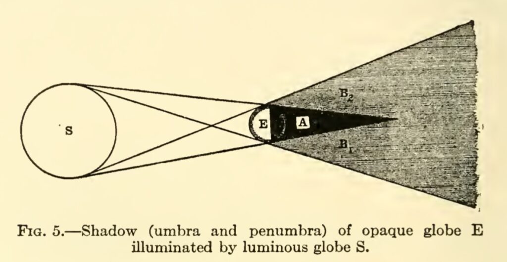
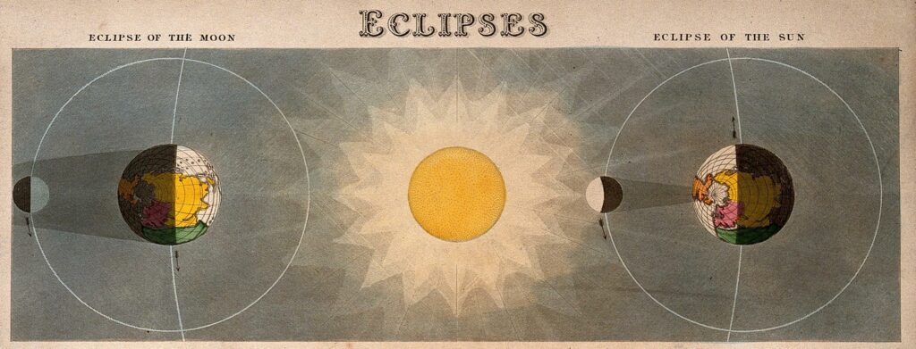
The Sun is our ultimate light source on Earth. The side of the Earth facing the Sun is bathed in sunlight, due to our rotation this side changes continuously. The side which faces the Sun has the day, and the other side is the night, in the shadow of the entire Earth. The sun being an extended source (and not a point source), the Earth’s shadow had both umbra and penumbra. Umbra is the region where no light falls, while penumbra is a region where some light falls. In case of an extended source like the Sun, this would mean that light from some part of the Sun does fall in the penumbra. Occasionally, when the Moon falls in this shadow we get the lunar eclipse. Sometimes it is total lunar eclipse, while many other times it is partial lunar eclipse. Total lunar eclipse occurs when the Moon falls in the umbra, while partial one occurs when it is in penumbra. On the other hand, when the Moon is between the Earth and the Sun, we get a solar eclipse. The places where the umbra of the Moon’s shadow falls, we get total solar eclipse, which is a narrow path on the surface of the Earth, and places where the penumbra falls a partial solar eclipse is visible. But how big is this shadow? How long is it? How big is the umbra and how big is the penumbra? We will do some rough calculations, to estimate these answers and some more to understand the phenomena of eclipses.

We will start with a reasonable assumption that both the Sun and the Earth as spheres. The radii of the Sun, the Earth and the Moon, and the respective distances between them are known. The Sun-Earth-Moon system being a dynamic one, the distances change depending on the configurations, but we can assume average distances for our purpose.

[The image above is interactive, move the points to see the changes. This construction is not to scale!. The simulation was created with Cinderella ]

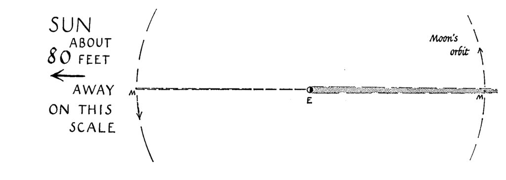
The diameter of the Earth is approximately 12,742 kilometers, and the diameter of the Sun is about 1,391,000 kilometers, hence the ratio is about 109, while the distance between the Sun and the Earth is about 149 million kilometers. A couple of illustrations depicting it on the correct scale.

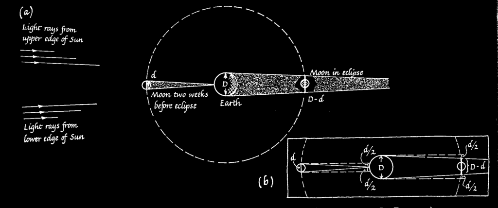
The Sun’s (with center A) diameter is represented by DF, while EG represents Earth’s (with center C) diameter. We connect the centers of Earth and Sun. The umbra will be limited in extent in the cone with base EG and height HC, while the penumbra is infinite in extent expanding from EG to infinity. The region from umbra to penumbra changes in intensity gradually. If we take a projection of the system on a plane bisecting the spheres, we get two similar triangles HDF and HEG. We have made an assumption that our properties of similar triangles from Euclidean geometry are valid here.

In the schematic diagram above (not to scale) the umbra of the Earth terminates at point H. Point H is the point which when extended gives tangents to both the circles. (How do we find a point which gives tangents to both the circles? Is this point unique?). Now by simple ratio of similar triangles, we get

$$
\frac{DF}{EG} = \frac{HA}{HC} = \frac{HC+AC}{HC}
$$

Therefore,

$$
HC = \frac{AC}{DF/EG -1}
$$

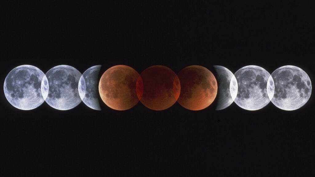
Now, $DF/EG = 109$, and $AC$ = 149 million km, substituting the values we get the length of the umbra $HC \approx$ 1.37 million km. The Moon, which is at an average distance of 384,400 kilometers, sometimes falls in this umbra, we get a total lunar eclipse. The composite image of different phases of a total lunar eclipse below depicts this beautifully. One can “see” the round shape of Earth’s umbra in the central three images of the Moon (red coloured) when it is completely in the umbra of the Earth (Why is it red?).

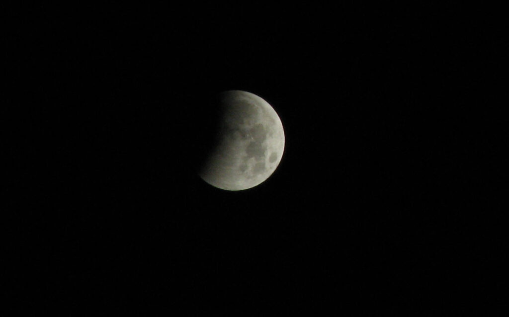
When only a part of umbra falls on the moon we get a partial lunar eclipse as shown below. Only a part of Earth’s umbra is on the Moon.

So if the moon was a bit further away, lets say at 500,000 km, we would not get a total solar eclipse. Due to a tilt in Moon’s orbit not every new moon is an eclipse meaning that the Moon is outside both the umbra and the penumbra.

The observations of the lunar eclipse can also help us estimate the diameter of the Moon.

Similar principle applies (though the numbers change) for solar eclipses, when the Moon is between the Earth and the Sun. In case of the Moon, ratio of diameter of the Sun and the Moon is about 400. With the distance between them approximately equal to the distance between Earth and the Sun. Hence the length of the umbra using the above formula is 0.37 million km or about 370,000 km. This makes the total eclipse visible on a small region of Earth and is not extended, even the penumbra is not large (How wide is the umbra and the penumbra of the moon on the surface of the Earth?).

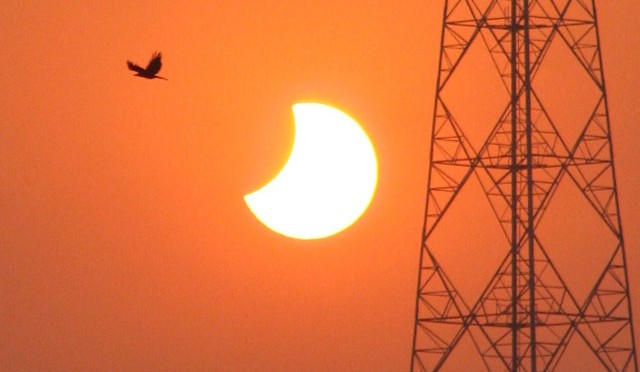
When only penumbra is falling on a given region, we get the partial solar eclipse.

You can explore when solar eclipse will occur in your area (or has occurred) using the Solar Eclipse Explorer.

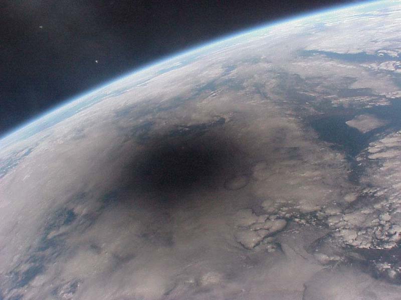
This is how the umbra of the Moon looks like from space.

And same thing would happen to a globe held in sunlight, its shadow would be given by the same ratio.

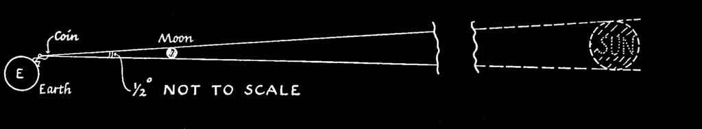
Thus we see that the numbers are almost matched to give us total solar eclipse, sometimes when the moon is a bit further away we may also get what is called the annular solar eclipse, in which the Sun is not covered completely by the Moon. Though the total lunar eclipses are relatively common (average twice a year) as compared to total solar eclipses (once 18 months to 2 years). Another coincidence is that the angular diameters of the Moon and the Sun are almost matched in the sky, both are about half a degree (distance/diameter ratio is about 1/110). Combined with the ratio of distances we are fortunate to get total solar eclipses.

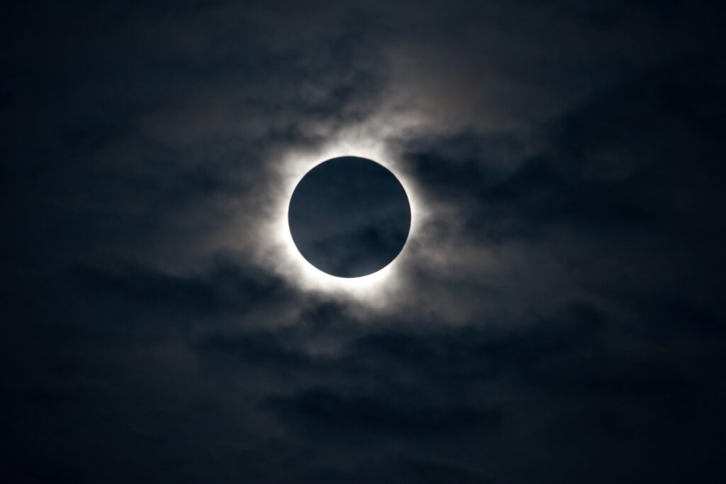
Seeing and experiencing a total solar eclipse is an overwhelming experience even when we have an understanding about why and how it happens. More so in the past, when the Sun considered a god, went out in broad daylight. This was considered (and is still considered by many) as a bad omen. But how did the ancient people understand eclipses? There is a certain periodicity in the eclipses, which can be found out by collecting large number of observations and finding patterns in them. This was done by ancient Babylonians, who had continuous data about eclipses from several centuries. Of course sometimes the eclipse will happen in some other part of the Earth and not be visible in the given region, still it could be predicted. To be able to predict eclipses was a great power, and people who could do that became the priestly class. But the Babylonians did not have a model to explain such observations. Next stage that came up was in ancient Greece where models were developed to explain (and predict) the observations. This continues to our present age.

The discussion we have had applies in the case when the light source (in this case the Sun) is larger than the opaque object (in this case the Earth). If the the light source is smaller than the object what will happen to the umbra? It turns out that the umbra is infinite in extent. You see this effect when you get your hand close to a flame of candle and the shadow of your hand becomes ridiculously large! See what happens in the interactive simulation above.

References

James Southhall Mirrors, Prisms and Lenses (1918) Macmillan Company

Eric Rogers Physics for the Inquiring Mind (1969) Princeton

July 14, 2023 The Mitr

Remarkable Curves 1: The Straight Line and the Circle

The Straight Line and the circle

(Note: All the images are interactive, move the points around to see. Dynamic mathematics interactive web page with Cinderella )

A moving point describes a straight line when it passes from one
position to another along the shortest possible path. A straight line
can be drawn with the help of a ruler; when a pencil runs along the
edge of a ruler it leaves a trace on the paper in the form of a
straight line.

When a point moves on a surface at a constant distance from another
fixed point on the same surface it describes a circle. Because of this
property of the circle we are able to draw a circle with the help of
compasses.

The straight line and the circle are the simplest and at the same time
the most remarkable curves as far as their properties are concerned.

You are no doubt more familiar with these two curves than with
others. But you should not imagine that you know all of the most
important properties of straight lines and curves. For example, you
may not know that if the vertices of the triangles $ABC$ and $AB’C’$
lie on three straight lines intersecting at the point $S$ (Fig. 1),
the three points of intersection $M$, $K$, $L$ of the corresponding
sides of the triangles, the sides $AB$ and $A’B’$, $BC$ and $B’C’$,
and $AC$ and $A’C’$, must be collinear, that is, they lie on a single
straight line.

(Note: this image below is interactive, move the points to see the dynamic change!)

You are sure to know that a point $M$ moving in a plane equidistantly
from two fixed points, say $F_1$, and $F_2$, of the same plane, that
is, so that $MF_{1}= MF_{2}$, describes a straight line (Fig. 2).

But you might find it difficult to answer the question:

What type of curve will point $M$ describe if the distance of $M$ from
$F_1$, is a certain number of times greater than that from $F_2$ (for
instance, in Fig. 3 it is twice as great)?

The curve turns out to be a circle. Hence if the point $M$ moves in a
plane so that the distance of $M$ from one of the fixed
points. $F_{1}$ or $F_{2}$, in the same plane is always proportional
to the distance from the other fixed point, that is

$$
MF_{1} = k \times MF_{2}
$$

then $M$ describes either a straight line (when the factor of
proportionality is unity) or a circle (when the factor of
proportionality is other than unity).

This is a post to create interactive mathematics elements using Cinderella a Free Software alternative to GeoGebra which is no longer a Free Software. The files have been exported from Cinderella at html interactives)

December 3, 2022December 5, 2022 The Mitr

What is the mathematical significance of the constant C in an indefinite integral?

As we had seen in an earlier post, calculus bottleneck, calculus presents one of the most difficult topics for the students in higher mathematics. But the problem is not just limited to the students. Teachers feel it too. Too often the emphasis is given on how to solve integration and differentiation problems using “rules” and “methods” while the essence of what is happening is lost. Recently, I asked this question in an interview to a mathematics teacher who was teaching indefinite integration. This teacher had almost a decade of experience in teaching mathematics at +2 level. The teacher tried to answer this question by using an example of the function $x^{2} + 5 $. Now when we take the derivative of this function, we get

\[ \dv{ (x^{2} + 5)}{x} = \dv{x^{2}}{x} + \dv{5}{x} = 2x \]

as derivative of a constant (5 on our case) is 0). Now the teacher tried to argue, that integration is the reverse of the derivative), so

\[ \int 2x \, \dd x = \frac{2x^{2}}{2} + C = 2x + C \]

After this the teacher tried to argue this $ C $ represents the constant term (5) in our function $x^{2} + 5 $. He tried to generalise the result, but he was thinking concretely in terms of the constant in the form of the numbers in the function. The teacher could understand the mechanism of solving the problem, but was not able to explain in clear mathematical terms, why the constant $ C $ was required in the output of the indefinite integral. This difficulty, I think, partly arose because the teacher only thought in terms solving integrals and derivatives in a particular way, and knew about the connection between the two, but not in a deep way. He did in a way understood the essence of the constant $ C $, but was not able to understand my question as a general question and hence replied only in terms of concrete functions. Even after repeated probing, the teacher could not get the essence of the question:

why do we add a constant term to the result of the indefinite integral?

To put it in another words, he was not able to generalise an abstract level of understanding from the examples that were discussed. The teacher was thinking only in terms of symbol manipulation rules which are sufficient for problem solving of these types. For example, look at the corresponding rules for differentiation and integration of the function $x^{n} $.

\[ \dv{x^{n}}{x} = n x^{n-1} \iff \int x^{n} \dd x = \frac{x^{n+1}}{n} + C \]

Thus, we see according to above correspondence that adding any extra constant $ C $ to the derivative formula will not affect it. So the teacher claimed it is this constant which appears in the integration rule as well. In a way this is a sort of correct explanation, but it does not get to the mathematical gist of why it is so. What is the core mathematical idea that this constant $ C $ represents.

Another issue, I think, was the lack of any geometrical interpretation during the discussion. If you ask, what is the geometrical interpretation of the derivative you will get a generic answer along the lines: “It is the tangent to the curve” and for integration the generic answer is along the lines “It is the area under the curve”. Both these answers are correct, but how do these connect to the equivalence above? What is the relationship between the tangent to the curve and area under the curve which allows us to call the integral as the anti-derivative (or is the derivative an anti-integral?). I think to understand these concepts better we have to use the geometrical interpretation of the derivative and the integral from their first definitions.

The basic idea behind the derivative is that it represents the rate of change of a function $ f $ at a given point. This idea, for an arbitrary function, can be defined (or interpreted) geometrically as:

The derivative of a function $ f $ at a point $ x_{0} $ is defined by the slope of the tangent to the graph of the function $ f $ at the point $x = x_{0} $.

The animation below shows how the slope of the tangent to the sine curve changes. Point $ B $ in the animation below plots the $ (x, m) $, where $ m $ is the slope of the tangent for the given value of $ x $. Can you mentally trace the locus of point $ B $? What curve is it tracing?

Now, the tangent to any point on a curve is unique. (Why is it so?) That means if one evaluates a derivative of a function at a point, it will be a unique result for that point.

This being cleared, now let us turn to the indefinite integral. One approach to understanding integration is to consider it as an inverse operation to the derivative, i.e. an anti-derivative.

An anti-derivative is defined as a function $ F(x) $ whose derivative equals an initial function $f (x) $:

\[ f(x)= \dv{ F(x)}{x} \]

Let us take an example of the function $ f(x) = 2x^{2} – 3x $. The differentiation of this function gives us its derivative $f'(x) = 4x – 3 $, and its integration gives us anti-derivative.
\[ F(x) = \frac{2}{3} x^{3} – \frac{3}{2} x^2 \]

This anti-derivative can be obtained by applying the known rules of differentiation in the reverse order. We can verify that the differentiation of the anti-derivative leads us to the original function.

\[ F'(x) = \frac{2}{3} 3 x^{2} – \frac{3}{2} 2 x = 2x^{2} – 3x \]

Now if add a constant to the function $ F(x) $, lets say number 4, we get a function $ G(x) = \frac{2}{3} x^{3} – \frac{3}{2} x^2 + 4 $. If we take the derivative of this function $ G(x) $, we still get our original function back. This is due to the fact that the derivative of a constant is zero. Thus, there can be any arbitrary constant added to the function $ F(x) $ and it will still be the anti-derivative of the original function $ f(x) $.

An anti-derivative found for a given function is not unique. If $ F (x) $ is an anti-derivative (for a function $ f $ ), then any function $ F(x)+C $, where $ C $ is an arbitrary constant, is also an anti-derivative for the initial function because
\[
\dv{[F(x)+C]}{x} = \dv{ F(x)}{x} + \dv{ C}{x}= \dv{ F(x) }
\]

But what is the meaning of this constant $ C $? This means, that each given function $ f (x) $ corresponds to a family of anti-derivatives, $ F (x) + C $. The result of adding a constant $ C $ to any function is that it shifts along the $ Y $-axis.

Thus what it means for our case of result of the anti-derivative, the resultant would be a family of functions which are separated by $ C$. For example, let us look at the anti-derivative of $ f (x) = \sin x $. The curves of anti-derivatives for this function are plotted in will be of the form

\[
F ( x ) = − \cos x + C
\]

A family of curves of the anti-derivatives of the function $ f (x) = \sin x = – \cos x $

And this is the reason for adding the arbitrary constant $ C$ to our result of the anti-derivative: we get a family of curves and the solution is not unique.

Now can we ever know the value of $ C$? Of course we can, but for this we need to know the some other information about the problem at hand. These can be initial conditions (values) of the variables or the boundary condition. Once we know these we can determine a particular curve (particular solution) from the family of curves for that given problem.

Numbers: Rational and Irrational

From Numbers: Rational and Irrational by Ivan Niven

July 6, 2021October 15, 2022 The Mitr

A complex systems approach to biology – a review of How Leopard Changed its Spots by Brian Goodwin

How the Leopard Changed it Spots by Brian Goodwin talks about a different approach to biology. After the genetic and molecular biology revolution 1950s onwards, increasingly the organism has been shifted out of focus in biology. Instead genes and their effect, genocentrism or neo-Darwninism, have taken the central stage. Everything in biology is seen as an “action” of genes in addition to natural selection. This translates to reductionism, everything is reduced to genes which are considered as the most fundamental units of life. This is the dominant approach in biology for some decades now. The terms such as “selfish gene” basically highlight this point. Such an approach sidelines the organism as a whole and its environment and highlights the genes alone. Good draws analogy of “word” of god seen as the final one in scriptures to the code alphabet in the genes, as if their actions and results are inevitable and immutable.
Goodwin in his work argues against such an approach using a complex systems perspective. In the process he also critiques what is an acceptable “explanation” in biology vis-a-vis other sciences. The explanation in biology typically is a historical one, in which features and processes are seen in the light of its inheritance and survival value of its properties. This “explanation” does not explain why certain forms are possible. Goodwin with examples establishes how action of genes alone cannot establish the form of the organism (morphogenesis). Genes only play one of the parts in morphogenesis, but are not solely responsible for it (which is how neo-Darwinist account argue). He cites examples from complex systems such as Belousov–Zhabotinsky reaction, ant colonies to establish the fact that in any system there are different levels of organisation. And there are phenomena, emergent phenomena, which cannot be predicted on the basis of the properties constituent parts alone. Simple interactions of components at lower level can give rise to (often) surprising properties at higher level. He is very clear that natural selection is universal (Darwin’s Dangerous Idea?!)

> What this makes clear is that there is nothing particularly biological about natural selection: it is simply a term used by biologists to describe the way in which one form replaces another as a result of their different dynamic properties. This is just a way of talking about dynamic stability, a concept used for a long time in physics and chemistry. We could, if we wished, simply replace the term natural selection with dynamic stabilization, the emergence of the stable states in a dynamic system. p. 53

Goodwin uses the term morphogenetic space to convey the possible shape space that an organism can occupy. Thus seen from a complex systems perspective, the various unit of the organism interact to generate the form of the organism. Natural selection then acts as a coarse sieve on these forms with respect to the environmental landscape. The “aim” of the organism is not the climb the fitness lanscape but to achieve dynamic stability.

> The relevant notion for the analysis of evolving systems is dynamic stability: A necessary (though by no means sufficient} condition for the survival of a species is that its life cycle be dynamically stable in a particular environment. This stability refers to the dynamics of the whole cycle, involving the whole organism as an integrated system that is itself integrated into a greater system, which is its habitat. p. 179

Goodwin takes examples of biological model systems and shows how using mathematical models we can generate their forms. Structure of acetabularia (a largish ~1 inch single cell algae), the structure of eye, the Fibonacci pattern seen in many flower structures being the main examples. Also, how the three basic forms of leaf arrangement can be generated by variations on a theme in the morphospace are discussed in detail. The model shows that three major forms are the most probable ones, which is actually substantiated by observations in nature. In these examples, an holistic approach is taken in which genes, competition and natural selection only play a part are not the main characters but are interacting and cooperating with levels of organisation of the organism, environmental factors in the drama of life.

> Competition has no special status in biological dynamics, where what is important is the pattern of relationships and interactions that exist and how they contribute to the behavior of the system as an integrated whole.The problem of origins requires an understanding of how new levels of order emerge from complex patterns of interaction and what the properties of these emergent structures are in terms of their robustness to perturbation and their capacity for self-maintenance. Then all levels of order and organization are recognized as equally important in understanding the behavior of living systems, and the reductionist insistence on some basic material level of cause and explanation, such as molecules and genes, can be recognized as an unfortunate fashion or prejudice that is actually bad science. P.181

Since I am already a believer of the complex systems perspective, I was aware of some of the arguments in this book, but the particular worked examples and their interpretation for biology was a fresh experience.

July 23, 2020August 22, 2023 The Mitr

The Calculus Bottleneck

What if someone told you that learners in high-school don’t actually need calculus as a compulsory subject for a career in STEM? Surely I would disagree. After all, without calculus how will they understand many of the topics in the STEM. For example basic Newtonian mechanics? Another line of thought that might be put forth is that calculus allows learners to develop an interest in mathematics and pursue it as a career. But swell, nothing could be farther from truth. From what I have experienced there are two major categories of students who take calculus in high school. The first category would be students who are just out of wits about calculus, its purpose and meaning. They just see it as another infliction upon them without any significance. They struggle with remembering the formulae and will just barely pass the course (and many times don’t). These students hate mathematics, calculus makes it worse. Integration is opposite of differentiation: but why teach it to us?

The other major category of students is the one who take on calculus but with a caveat. They are the ones who will score in the 80s and 90s in the examination, but they have cracked the exam system per se. And might not have any foundational knowledge of calculus. But someone might ask how can one score 95/100 and still not have foundational knowledge of the subject matter? This is the way to beat the system. These learners are usually drilled in solving problems of a particular type. It is no different than chug and slug. They see a particular problem – they apply a rote learned method to solve it and bingo there is a solution. I have seen students labour “problem sets” — typically hundreds of problems of a given type — to score in the 90s in the papers. This just gives them the ability to solve typical problems which are usually asked in the examinations. Since the examination does not ask for questions based on conceptual knowledge – it never gets tested. Perhaps even their teachers if asked conceptual questions will not be able to handle them — it will be treated like a radioactive waste and thrown out — since it will be out of syllabus.
There is a third minority (a real minority, and may not be real!, this might just be wishful thinking) who will actually understand the meaning and significance of the conceptual knowledge, and they might not score in the 90s. They might take a fancy for the subject due to calculus but the way syllabus is structured it is astonishing that any students have any fascination left for mathematics. Like someone had said: the fascination for mathematics cannot be taught it must be caught. And this is exactly what MAA and NCTM have said in their statement about dropping calculus from high-school.

What the members of the mathematical community—especially those in the Mathematical Association of America (MAA) and the National Council of Teachers of Mathematics (NCTM)—have known for a long time is that the pump that is pushing more students into more advanced mathematics ever earlier is not just ineffective: It is counter-productive. Too many students are moving too fast through preliminary courses so that they can get calculus onto their high school transcripts. The result is that even if they are able to pass high school calculus, they have established an inadequate foundation on which to build the mathematical knowledge required for a STEM career. (emphasis added)

The problem stems from the fact that the foundational topics which are prerequisites for calculus are on shaky grounds. No wonder anything build on top of them is not solid. I remember having very rudimentary calculus in college chemistry, when it was not needed and high-flying into physical meaning of derivatives in physics which was not covered enough earlier. There is a certain mismatch between the expectations from the students and their actual knowledge of the discipline as they come to college from high-school.

Too many students are being accelerated, short-changing their preparation in and knowledge of algebra, geometry, trigonometry, and other precalculus topics. Too many students experience a secondary school calculus course that drills on the techniques and procedures that will enable them to successfully answer standard problems, but are never challenged to encounter and understand the conceptual foundations of calculus. Too many students arrive at college Calculus I and see a course that looks like a review of what they learned the year before. By the time they realize that the expectations of this course are very different from what they had previously experienced, it is often too late to get up to speed.

Though they conclude that with enough solid conceptual background in these prerequisites it might be beneficial for the students to have a calculus course in the highschool.

October 25, 2019August 22, 2023 The Mitr

Experiments, Data and Analysis

There are many sad stories of students, burning to carry out an experimental project, who end up with a completely unanalysable mishmash of data. They wanted to get on with it and thought that they could leave thoughts of analysis until after the experiment. They were wrong. Statistical analysis and experimental design must be considered together…
Using statistics is no insurance against producing rubbish. Badly used, misapplied statistics simply allow one to produce quantitative rubbish rather than qualitative rubbish.
– Colin Robson (Experiment, Design and Statistics in Psychology)

February 14, 2019August 22, 2023 The Mitr

The logician, the mathematician, the physicist, and the engineer

The logician, the mathematician, the physicist, and the engineer. “Look at this mathematician,” said the logician. “He observes that the first ninety-nine numbers are less than hundred and infers hence, by what he calls induction, that all numbers are less than a hundred.”
“A physicist believes,” said the mathematician, “that 60 is divisible by all numbers. He observes that 60 is divisible by 1, 2, 3, 4, 5, and 6. He examines a few more cases, as 10, 20, and 30, taken at random as he says. Since 60 is divisible also by these, he considers the experimental evidence sufficient.”
“Yes, but look at the engineers,” said the physicist. “An engineer suspected that all odd numbers are prime numbers. At any rate, 1 can be considered as a prime number, he argued. Then there come 3, 5, and 7, all indubitably primes. Then there comes 9; an awkward case, it does not seem to be a prime number. Yet 11 and 13 are certainly primes. ‘Coming back to 9’ he said, ‘I conclude that 9 must be an experimental error.'”
– George Polya (Induction and Analogy – Mathematics of Plausible Reasoning – Vol. 1, 1954)

February 12, 2019August 22, 2023 The Mitr

On mathematics

Mathematics is regarded as a demonstrative science. Yet this is only one of its aspects. Finished mathematics presented in a finished form appears as purely demonstrative, consisting of proofs only. Yet mathematics in the making resembles any other human knowledge in the making. You have to guess a mathematical theorem before you prove it; you have to guess the idea of the proof before you carry through the details. You have to combine observations and follow analogies; you have to try and try again. The result of the mathematician’s creative work is demonstrative reasoning, a proof; but the proof is discovered by plausible reasoning, by guessing. If the learning of mathematics reflects to any degree the invention of mathematics, it must have a place for guessing, for plausible inference.
– George Polya (Induction and Analogy – Mathematics of Plausible Reasoning – Vol. 1, 1954)

January 25, 2019August 22, 2023 The Mitr

Unreal and Useless Problems

We had previously talked about problem with contexts given in mathematics problems. This is not new, Thorndike in 1926 made similar observations.
Unreal and Useless Problems
In a previous chapter it was shown that about half of the verbal problems given in standard courses were not genuine, since in real life the answer would not be needed. Obviously we should not, except for reasons of weight, thus connect algebraic work with futility. Similarly we should not teach the pupil to solve by algebra problems which in reality are better solved otherwise, for example, by actual counting or measuring. Similarly we should not set him to solve problems which are silly or trivial, connecting algebra in his mind with pettiness and folly, unless there is some clear, counterbalancing gain.
This may seem beside the point to some teachers, ”A problem is just a problem to the children,” they will say,
“The children don’t know or care whether it is about men or fairies, ball games or consecutive numbers.” This may be largely true in some classes, but it strengthens our criticism. For, if pupils^do not know what the problem is about, they are forming the extremely bad habit of solving problems by considering only the numbers, conjunctions, etc., regardless of the situation described. If they do not care what it is about, it is probably because the problems encountered have not on the average been worth caring about save as corpora vilia for practice in thinking.
Another objection to our criticism may be that great mathematicians have been interested in problems which are admittedly silly or trivial. So Bhaskara addresses a young woman as follows: ”The square root of half the number of a swarm of bees is gone to a shrub of jasmine; and so are eight-ninths of the swarm: a female is buzzing to one remaining male that is humming within a lotus, in which he is confined, having been allured to it by its fragrance at night. Say, lovely woman, the number of bees.” Euclid is the reputed author of: ”A mule and a donkey were going to market laden with wheat. The mule said,’If you gave me one measure I should carry twice as much as you, but if I gave you one we should bear equal burdens.’ Tell me, learned geometrician, what were their burdens.” Diophantus is said to have included in his preparations for death the composition of this for his epitaph : ” Diophantus passed one-sixth of his life in childhood one-twelfth in youth, and one-seventh more as a bachelor. Five years after his marriage was born a son, who died four years before his father at half his father’s age.”
My answer to this is that pupils of great mathematical interest and ability to whom the mathematical aspects of these problems outweigh all else about them will also be interested in such problems, but the rank and file of pupils will react primarily to the silliness and triviality. If all they experience of algebra is that it solves such problems they will think it a folly; if all they know of Euclid or Diophantus is that he put such problems, they will think him a fool. Such enjoyment of these problems as they do have is indeed compounded in part of a feeling of superiority.
– From Thorndike et al. The Psychology of Algebra 1926

Temet Nosce

Know Thyself Too…

mathematics